5. Performance analysis
- 5.1 Available Performance Analysis Tools
- 5.2 Cray Performance Analysis Tool (CrayPAT)
- 5.3 Allinea MAP
- 5.2 General hints for interpreting profiling results
5.1 Available Performance Analysis Tools
All Cray XE machines come with the Cray Performance Tools (module "perftools") installed. These tools include:
- Cray Performance Analysis Tool (CrayPAT).
- PAPI hardware counters.
- Apprentice2 performance visualisation suite.
CrayPAT provides the interface to using all these tools.
Some systems will have addtional, third-party, tools available. These can include:
- Allinea MAP
- Vampir
- Scalasca
HECToR also has Allinea MAP, Scalasca and VampiTrace performance analysis tools installed. We provide details below on how to use MAP. For more information on the other tools please see the appropriate online documentation:
5.2 Cray Performance Analysis Tool (CrayPAT)
CrayPAT consists of two command line tools which are used to profile your code: 'pat_build' adds instrumentation to your code so that when you run the instrumented binary the profiling information is stored on disk; 'pat_report' reads the profiling information on disk and compiles it into human-readable reports.
CrayPAT can perform two types of performance analysis: sampling experiments and tracing experiments. A sampling experiment probes the code at a predefined interval and produces a report based on these statistics. A tracing experiment explicitly monitors the code performance within named routines. Typically, the overhead associated with a tracing experiment is higher than that associated with a sampling experiment but provides much more detailed information. The key to getting useful data out of a sampling experiment is to run your profiling for a representitive length of time.
Detailed documentation on CrayPAT is available from Cray:
5.2.1 Instrumenting a code with pat_build
Often the best way to to analyse the performance is to run a sampling experiment and then use the results from this to perform a focussed tracing experiment. In fact, CrayPAT contains the functionality for automating this process - known as Automatic Profiling Analysis (APA).
The example below illustrates how to do this.
5.2.1.1 Example: Profiling the CASTEP Code
Here is a step-by-step example to instrumenting and profiling the performance of a code (CASTEP) using CrayPAT.
The first step is to compile your code with the profiling tools attached. First load the Cray 'perftools' module with:
module add perftools
Next, compile the CASTEP code in the standard way on the "work" filesystem (which is accessible on the compute nodes). Once you have the CASTEP executable you need to instrument it for a sampling experiment. The following command will produce the 'castep+samp' instrumented executable:
pat_build -O apa -o castep+samp castep
Run your program as you usually would in the batch system at your site. Here is an example job submission script for a 32-core per node (Interlagos) system.
#!/bin/bash --login
#PBS -N bench4_il
#PBS -l mppwidth=1024
#PBS -l mppnppn=32
#PBS -l walltime=1:00:00
# Set this to your budget code
#PBS -A budget

# Switch to the directory you submitted the job from
cd $PBS_O_WORKDIR

# Load the perftools module
module add perftools

# Run the sampling experiment
CASTEP_EXEDIR=/work/user/software/CASTEP/bin
aprun -n 1024 -N 32 $CASTEP_EXEDIR/castep+samp input
When the job completes successfully the directory you submitted the job from will either contain an *.xf file (if you used a small number of cores) or a directory (for large core counts) with a name something like:
castep+samp+25370-14s
The actual name is dependent on the name of your instrumented executable and the process ID. In this case we used 1024 cores so we have got a directory.
The next step is to produce a basic performance report and also the input for 'pat_build' to create a tracing experiment. This is done (usually interactively) by using the 'pat_report' command (you must have the 'perftools' module loaded to use the pat_report command). In our example we would type:
pat_report -o castep_samp_1024.pat castep+samp+25370-14s
this will produce a text report (in castep_samp_1024.pat) listing the various routines in the program and how much time was spent in each one during the run (see below for a discussion on the contents of this file). It also produces a castep+samp+25370-14s.ap2 file and a castep+samp+25370-14s.apa file:
- The *.ap2 file can be used with the Apprentice2 visualisation tool to get an alternative view of the code performance.
- The *.apa file can be used as the input to "pat_build" to produce a tracing experiment focussed on the routines that take most time (as determined in the previous sampling experiment). We illustrate this below.
For information on interpreting the results in the sampling experiment text report, see the section below.
To produce a focussed tracing experiment based on the results from the sampling experiment above we would use the 'pat_build' command with the *.apa file produced above. (Note, there is no need to change directory to the directory containing the original binary to run this command.)
pat_build -O castep+samp+25370-14s.apa -o castep+apa
This will generate a new instrumented version of the CASTEP executable (castep+apa) in the current working directory. You can then submit a job (as outlined above) making sure that you reference this new executable. This will then run a tracing experiment based on the options in the *.apa file.
Once again, you will find that your job generates a *.xf file (or a directory) which you can analyse using the 'pat_report' command. Please see the section below for information on analysing tracing experiments.
5.2.2 Analysing profile results using pat_report
The 'pat_report' command is able to produce many different profile reports from the profile data. You can select the type of pre-defined report options with the -O flag to 'pat_report'. A selection of the most generally useful pre-defined report types are:
- ca+src - Show the callers (bottom-up view) leading to the routines that have a high use in the report and include source code line numbers for the calls and time-consuming statements.
- load_balance - Show load-balance statistics for the high-use routines in the program. Parallel processes with minimum, maximum and median times for routines will be displayed. Only available with tracing experiments.
- mpi_callers - Show MPI message statistics. Only available with tracing experiments
Multiple options can be specified to the -O flag if they are separated by commas. For example:
pat_report -O ca+src,load_balance -o castep_furtherinfo_1024.pat castep+samp+25370-14s
You can also define your own custom reports using the -b and -d flags to 'pat_report'. Details on how to do this can be found in the 'pat_report' documentation and man pages. The output from the pre-defined report types (described above) show the settings of the -b and -d flags that were used to generate the report. You can use these examples as the basis for your own custom reports.
Below, we show examples of the output from sampling and tracing experiments for the pure MPI version of CASTEP. A report from your own code will differ in the routines and times shown. Also, if your code uses OpenMP threads, SHMEM, or CAF/UPC then you will also see different output.
5.2.2.1 Example: results from a sampling experiment on CASTEP
In a sampling experiment, the main summary table produced by 'pat_report' will look something like (of course, your code will contain different functions and subroutines):
Table 1:  Profile by Function

 Samp%  |  Samp  |  Imb.  |  Imb.  |Group
        |        |  Samp  | Samp%  | Function
        |        |        |        |  PE=HIDE

 100.0% | 6954.6 |     -- |     -- |Total
|----------------------------------------------------------------------
|  46.0% | 3199.8 |     -- |     -- |MPI
||---------------------------------------------------------------------
||  12.9% |  897.0 |  302.0 |  25.6% |mpi_bcast
||  12.9% |  896.4 |   78.6 |   8.2% |mpi_alltoallv
||   8.7% |  604.2 |  139.8 |  19.1% |MPI_ALLREDUCE
||   5.4% |  378.6 | 1221.4 |  77.5% |MPI_SCATTER
||   4.9% |  341.6 |  320.4 |  49.2% |MPI_BARRIER
||   1.1% |   75.8 |  136.2 |  65.2% |mpi_gather
||=====================================================================
|  38.8% | 2697.9 |     -- |     -- |USER
||---------------------------------------------------------------------
||   9.4% |  652.1 |  171.9 |  21.2% |comms_transpose_exchange.3720
||   6.0% |  415.2 |   41.8 |   9.3% |zgemm_kernel_n
||   3.4% |  237.6 |   29.4 |  11.2% |zgemm_kernel_l
||   3.1% |  215.6 |   24.4 |  10.3% |zgemm_otcopy
||   1.7% |  119.8 |   20.2 |  14.6% |zgemm_oncopy
||   1.3% |   92.3 |   11.7 |  11.4% |zdotu_k
||=====================================================================
|  15.2% | 1057.0 |     -- |     -- |ETC
||---------------------------------------------------------------------
||   2.0% |  140.5 |   32.5 |  19.1% |__ion_MOD_ion_q_recip_interpolation
||   2.0% |  139.8 |  744.2 |  85.5% |__remainder_piby2
||   1.1% |   78.3 |   32.7 |  29.9% |__ion_MOD_ion_apply_and_add_ylm
||   1.1% |   73.5 |   35.5 |  33.1% |__trace_MOD_trace_entry
|======================================================================
You can see that CrayPAT splits the results from a sampling experiment into three sections:
- MPI - Samples accumulated in message passing routines
- USER - Samples accumulated in user routines. These are usually the functions and subroutines that are part of your program.
- ETC - Samples accumulated in library routines.
The first two columns indicate the % and number of samples (mean of samples computed across all parallel tasks) and indicate the functions in the program where the sampling experiment spent the most time. Columns 3 and 4 give an indication of the differences between the minimum number of samples and maximum number of samples found across different parallel tasks. This, in turn, gives an indication of where the load-imbalance in the program is found. Of course, it may be that load imbalance is found in routines where insignificant amounts of time are spent. In this case, the load-imbalance may not actually be significant (for example, the large imbalance time seen in 'mpi_gather' in the example above.
In the example above - the largest amounts of time seem to be spent in the MPI routines: mpi_bcast, mpi_alltoallv and MPI_ALLREDUCE and in the program routines: comms_transpose_exchange and the LAPACK routine 'zgemm'.
To narrow down where these time consuming calls are in the program we can use the 'ca+src' report option to 'pat_report' to get a view of the split of samples between the different calls to the time consuming routines in the program.
pat_report -O ca+src -o castep_calls_1024.pat castep+samp+25370-14s
An extract from the the report produced by the above command looks like
Table 1:  Profile by Function and Callers, with Line Numbers

 Samp%  |  Samp  |Group
        |        | Function
        |        |  Caller
        |        |   PE=HIDE

 100.0% | 6954.6 |Total
|--------------------------------------------------------------------------------------
--snip--
|  38.8% | 2697.9 |USER
||-------------------------------------------------------------------------------------
||   9.4% |  652.1 |comms_transpose_exchange.3720
|||------------------------------------------------------------------------------------
3||   3.7% |  254.4 |__comms_MOD_comms_transpose_n:comms.mpi.F90:line.17965
4||        |        | __comms_MOD_comms_transpose:comms.mpi.F90:line.17826
5||        |        |  __fft_MOD_fft_3d:fft.fftw3.F90:line.482
6||   3.1% |  215.0 |   __basis_MOD_basis_real_recip_reduced_one:basis.F90:line.4104
7||        |        |    __wave_MOD_wave_real_to_recip_wv_bks:wave.F90:line.24945
8||        |        |     __pot_MOD_pot_nongamma_apply_wvfn_slice:pot.F90:line.2640
9||        |        |      __pot_MOD_pot_apply_wvfn_slice:pot.F90:line.2550
10|        |        |       __electronic_MOD_electronic_apply_h_recip_wv:electronic.F90:line.4364
11|        |        |        __electronic_MOD_electronic_apply_h_wv:electronic.F90:line.4057
12|   3.0% |  211.4 |         __electronic_MOD_electronic_minimisation:electronic.F90:line.1957
13|   3.0% |  205.6 |          __geometry_MOD_geom_get_forces:geometry.F90:line.6299
14|   2.8% |  195.2 |           __geometry_MOD_geom_bfgs:geometry.F90:line.2199
15|        |        |            __geometry_MOD_geometry_optimise:geometry.F90:line.1051
16|        |        |             MAIN__:castep.f90:line.1013
17|        |        |              main:castep.f90:line.623
--snip--
This indicates that (in the USER routines) the part of the 'comms_transpose_exchange' routine in which the program is spending most time is around line 3720 (in many cases the time-consuming line will be the start of a loop). Furthermore, we can see that approximately one third of the samples in the routine (3.7%) are originating from the call to 'comms_transpose_exchange' in the stack shown. Here, it looks like they are part of the geometry optimisation section of CASTEP. The remaining two-thirds of the time will be indicated further down in the report.
In the original report (castep_samp_1024.pat) we also set a table reporting on the wall clock time of the program. The table reports the minimum, maximum and median values of wall clock time from the full set of parallel tasks. The table also lists the maximum memory usage of each of the parallel tasks:
Table 3:  Wall Clock Time, Memory High Water Mark

   Process  |  Process  |PE=[mmm]
      Time  |    HiMem  |
            | (MBytes)  |

 124.409675 |   100.761 |Total
|---------------------------------
| 126.922418 |   101.637 |pe.39
| 124.329474 |   102.336 |pe.2
| 122.241495 |   101.355 |pe.4
|=================================
If you see a very large difference in the minimum and maximum walltime for different parallel tasks it indicates that there is a large amount of load-imbalance in your code and it should be investigated more thouroughly.
5.2.2.2 Example: results from a tracing experiment on CASTEP
Coming soon…
5.2.3 Using hardware counters
CrayPAT also provides hardware counter data. CrayPAT supports both predefined hardware counter events and individual hardware counters. Please refer to the CrayPAT documatations for further details of the hardware counter events: http://docs.cray.com/
To use the hardware counter, you need to set the environment variable PAT_RT_HWPC in your in your job script when running your tracing experiment. For example:
export PAT_RT_HWPC=21
(on an Interlagos system) will specify the twenty-first of twenty-two predefined sets of hardware counter events to be measured and reported. This set provides information on floating-point operations, and cache performance.
Note that hardware counters are only supported with tracing experiments, not on sampling experiments. If you set PAT_RT_HWPC for a sampling experiment the instrumented executable will fail to run.
When you produce a profile report using 'pat_report', hardware counter information will automatically be included in the report if the PA_RT_HWPC environment variable was set when the experiment was run.
A full list of the predefined sets of counters can be found on the hardware counters man page on your execution site. To access the documentation, use:
man hwpc
5.2.3.1 Example: Hardware counter results from CASTEP
Coming soon…
5.3 Allinea MAP
Allinea MAP can be used to profile MPI code only - it does not support detailed profiling of OpenMP, SHMEM, CAF, or UPC. Profiling using Allinea MAP consists of four steps:
- Setup a MAP profiling version of your MPI library (generaly very simple).
- Re-compile your code linking the MAP MPI profiling library.
- Run your code to collecting profiling information.
- Visualise the profiling using the MAP Remote Client.
5.3.1 Create MAP profiling MPI library
You should first load the "allinea" module to give you access to all the MAP executables:
module add allinea
The command you use to create the profiling version of your MPI library differs depending whether you are linking statically or dynamically. On HECToR the default is to link statically so you should use the command for static libraries unless you are definitely linking dynamically.
For statically linked applications the command is "make-map-static-cray-libraries" and you need to supply a path for the tool to write the library files to. For example:
user@hector-xe6-5:~> mkdir map-libraries
user@hector-xe6-5:~> make-map-static-cray-libraries ./map-libraries
Created the MAP libraries in /home/t01/t01/user/map-libraries:
   libmap-sampler.a
   libmap-sampler-pmpi.a

To instrument a Cray XT/XK program, add these compiler options:
   compilation : -g (or '-G2' for native Cray fortran) (and -O3 etc.)
       linking : -L/home/t01/t01/user/map-libraries -lmap-sampler-pmpi \
                 -Wl,--undefined,allinea_init_sampler_now -lmap-sampler \
                 -lstdc++ -lgcc_eh -Wl,--whole-archive \
                 -lpthread -Wl,--no-whole-archive -Wl,--eh-frame-hdr

user@hector-xe6-5:~> ls -l ./map-libraries
total 1952
-rw-r--r-- 1 user t01       0 2013-09-30 11:48 conftest.err
-rw-r--r-- 1 user t01 1339458 2013-09-30 11:48 libmap-sampler.a
-rw-r--r-- 1 user t01  635782 2013-09-30 11:48 libmap-sampler-pmpi.a
If you are linking dynamically then you should use the "make-map-cray-libraries" command instead.
5.3.2 Re-compile code linking to MAP MPI libraries
Recompile your code with the "-g" flag to ensure debugging information is available for the profiler and then link using the set of options specified in the output from the "make-map-" command used above.
5.3.3 Run the profiling experiment
You can now run a job as normal to collect the profile information for your code. This involves writing a job submission script to run your code through MAP. MAP will produce a file containing all the profiling information which can then be examined using the Remote Client (as described below).
An example job submission script for running a profile across 32 MPI processes, 16 processes per node would be:
#!/bin/bash --login
#
#PBS -N map_test
#PBS -l mppwidth=64
#PBS -l walltime=1:0:0
#PBS -A t01

cd $PBS_O_WORKDIR

module add allinea

map -profile -n 32 -mpiargs "-N 16 -S 4 -d 2" myapp.exe
In this case the "-mpiargs" variable is used to pass additional command line arguments to the "aprun" command to specify the job placement.
This will produce a profile file with a name like:
myapp_32p_2013-09-30_11-07.map
You can specify a specific name for this output file using the "-output" option to "map" in you job script.
5.3.4 Visualise the profile data
In order to visualise the data you should download and install the Allinea Remote Client on your desktop from:
Once the client has downloaded, start it and you should see a startup screen similar to:
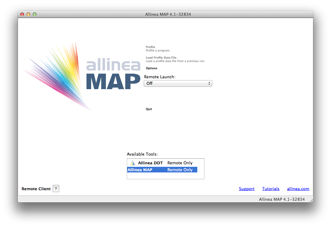
To set up the client to view results on HECToR you should select the "Remote Launch" pulldown and choose "Configure..." from the options. In the resulting dialogue box enter your HECToR username with the login details and the install location for MAP. For example:
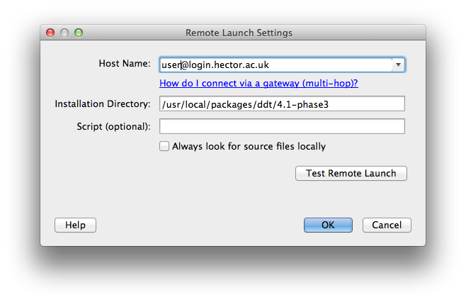
(If you do not have SSH keys set up to access your HECToR account you will need to enter your password when prompted.)
There are a number of different install locations on HECToR depending on which version of MAP you have downloaded. The current latest version (and default on HECToR) is 4.1.1 so you would enter the location
/usr/local/packages/ddt/4.1.1-phase3
()The 4.1-* version of MAP is availabel at /usr/local/packages/ddt/4.1-phase3 if you require it. This is the one illustrated in the example above.)
Once remote access has been successfully setup you should be returned to the startup screen. This time select "Load Profile Data File". You will be given a dialogue box where you can select your profile file from the HECToR filesystem. Once you have selected your file MAP will assemble your results and you can visualise your profile data. The MAP interface should look something like:
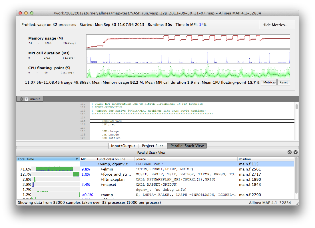
For more information on using the profiling interface see the Allinea documentation at:
5.4 General hints for interpreting profiling results
There are several general tips for using the results from the performance analysis:
- Look inside the routines where most of the time is spent to see if they can be optimised in any way - The "ct+src" report option can often be useful here to determine which regions of a function are using the most time.
- Look for load-imbalance in the code - This is indicted by a large difference in computing time between different parallel tasks.
- High values of time spent in MPI usually mean something wrong in the code - Load-imbalance, a bad communication pattern, or just not scaling to the used number of cores.
- High values of cache misses (seen via hardware counters) could mean a bad memory access in an array or loop - Examine the arrays and loops in the problematic function to see if they can be reorganised to access the data in a more cache-friendly way.
The Tuning section in this guide has a lot of information on how to optimise both serial and parallel code. Combining profiling information with the optimisation techniques is the best way to improve the performance of your code.
5.4.1 Spotting load-imbalance
By far the largest obstacle to scaling applications out to large numbers of parallel tasks is the presence of load-imbalance in the parallel code. Spotting the symptoms of load-imbalance in performance analysis are key to optimising the scaling performance of your code. Typical symptoms include:
- For MPI codes
- large amounts of time spent in MPI_BARRIER or MPI collectives (which include an implicit barrier).
- For OpenMP codes
- large amounts of time in "_omp_barrier" or "_omp_barrierp".
- For PGAS codes
- large amounts of time spent in sychronisation functions.
When running a CrayPAT tracing experiment with "-g mpi" the MPI time will be split into computation and "sync" time. A high "sync" time can indicate problems with load imbalance in an MPI code.
The location of the accumulation of load-imbalance time often gives an indication of where in your program the load-imbalance is occuring.
")