Good Practice Guide

HECToR Phase 3 (32-core)

Contents

• Introduction
• Who will benefit?
• What can I do to prepare?
• Architecture details
• Batch Submission
• Phase 3 Checklist
• NAG CSE Assistance
• References

Introduction

The theoretical peak performance and memory footprint of the service increases from around 370TF and 59TB in phase 2b to around 820TF and 90TB in phase 3.

This guide explains the key differences in software and architecture which will impact the operation and performance of codes in phase 3.

Who will benefit?

Peak performance of a node = 2.3 (GHz) * 8 (FLOPS/cycle) * 16 (Floating point units) = 294.4 GFLOPS/s.

When considered along with the decrease in the amount of memory per core from 1 1/3GB to 1GB, the introduction of the Interlagos chip can be seen as another step towards many-core computing, favouring applications with high computational intensity and low demand on data coming from main memory.

In going from phase 2a to 2b a HECToR node was increased from 4 cores to 24 cores; the increase at phase 3 to 32 cores is likely to be less of a significant change. However, optimizations to off-node MPI communications made during phase 2b will still pay off. The addition of an extra 10 cabinets increases the capability of the system so that jobs consisting of over 85,000 processes will be possible. At such scales Amdahl's law becomes very important, so only codes which minimize off-node MPI communications and with efficient I/O strategies will be able to perform such leading-edge capability science computations.

Another factor in ensuring your code makes good use of the machine is to benchmark different ways of running your application. Due to the complex, non-uniform nature of an XE6 node, there are many job placement possibilities to consider in running your jobs.

In summary, your code will be well placed to make good use of HECToR in phase 3 if it:

• makes use of tuned libraries whenever possible;
• has loops which compilers can vectorize easily;
• exploits temporal and spatial locality of data;
• minimizes off-node communications;
• has an appropriate I/O strategy;

If your code does not satisfy all of these conditions then the relative cost of running your jobs may increase, particularly if you wish to step up the scale of your runs. If you think that this will be the case, or if you would like help with any aspect of your code please contact the NAG CSE team via the helpdesk: support@hector.ac.uk, or check the training schedule for upcoming courses.

What can I do to prepare?

If performance does not match that seen during phase 2b then it is time to profile your code, considering the conditions outlined above for making good use of HECToR in phase 3. See the Good Practice Guide for Performance Measurement for tips on how to benchmark and profile your code. Please contact the NAG CSE team via the helpdesk: support@hector.ac.uk if you would like any help with this.

If profiling reveals that your code is not making good use of vector instructions then you might want to consider whether the section of code in question might be better replaced with a library call if possible. This will require some code restructuring, but it is a way to lift the burden of optimizing the most important parts of your code onto library developers, who focus on solving specific problems efficiently.

In the case that it is not possible or desirable to restructure your code to call library routines it is time to investigate why your loops are not vectorizing. This depends first of all on using the correct compiler flags:

Compiler	Suggested flags	Info flags
Cray	default*	-Omsgs,negmsgs
GNU	-O3	-ftree-vectorizer-verbose=2
PGI	-fast	-Minfo

Note that the Cray compiler is the default compiler available on login to the system in phase 3. The suggested flags are those which will cause the compiler to try to vectorize your loops (*note that you do not need to specify any optimization flags for the Cray compiler, default optimization is reasonably aggressive and will include vectorization). The info flags will provide some commentary on which loops were vectorized and which were not. For a discussion on vectorization, including some tips on writing vectorizable code see the "Instruction and data parallelism" section in our Good Practice Guide for Serial Code Optimisation.

If your code is still under-performing after making sure your important loops are vectorized, then it is a good idea to look at how your program is managing memory. Key to high performance is writing code with a high computational intensity and low demand on data coming from main memory. Making use of vector instructions is useless if the instructions are constantly waiting on data that is not present in a high level of the memory hierarchy. Making good use of temporal and spatial locality of data is also discussed in our Good Practice Guide for Serial Code Optimisation.

If the serial performance of your jobs is good, then the limiting factor is likely to be MPI communications and I/O. Several codes benefited from optimizations to reduce the number of off-node MPI messages during phase 2b, typically either by replacing MPI processes with OpenMP threads via the use of multithreaded libraries or adding OpenMP directives in hybrid jobs, or by making use of shared memory segments to make fewer, larger off-node MPI transactions. Techniques such as these are discussed in the Good Practice Guide for Parallel Code Optimisation.

If I/O is the bottleneck in your code then the likely solution will involve modifying the strategy for writing to files and/or utilizing MPI-IO. For a discussion of scalable I/O patterns and an overview of MPI-IO see the Good Practice Guide for I/O.

Finally, performance can be dramatically affected by the way in which you request and use resources in your job scripts, particularly if you are running hybrid jobs, or jobs which use shared memory segments. For advice on how to write job scripts in phase 3 see the batch submission section in this document.

Architecture details

A single node

The greatest difference compared to phase 2b is the architecture within a die. More resources are shared in the Interlagos chip compared to the phase 2b Magny-Cours chip. The 8 cores are paired into 4 "modules". Figure 1 provides a simple illustration of which resources are shared within a module.

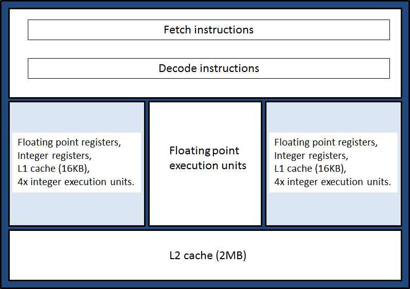
Figure 1. An Interlagos module. A module consists of two cores (shaded in light blue) which have independent L1 data cache, registers and execution units for integer operations. It shares L2 data cache, floating point execution units, and the hardware used to fetch and decode instructions.

Looking at a module in more detail, Figure 2 shows that the shared floating point unit consists of two 128-bit pipelines which are capable of grouping together as a single 256-bit pipeline. Thus each floating point unit is capable of executing two 128-bit SSE vector instructions or one 256-bit AVX add or multiply vector instruction per clock cycle. (See Good Practice Guide for Serial Code Optimisation for more information about vector instructions.) On top of SSE and AVX instructions there is a special 256-bit fused multiply-add instruction which effectively doubles the theoretical performance of the floating point units, and also has the benefit of improved accuracy compared with separate multiply followed by add instructions because the multiplication is not rounded before being used as input to the addition operation. Compilers will try to use this instruction where possible when vectorizing loops. It is important to realise two things about the new AVX and fused multiply-add instructions:

• A single 256-bit AVX instruction has the same throughput as two 128-bit SSE instructions operating in parallel: 4 double precision FLOPS per cycle, or 8 single precision FLOPS per cycle, which is the same as seen during phase 2b. However, one of the advantages of AVX instructions is that they are non-destructive, i.e. the result does not overwrite the contents of one of the input registers, because AVX instructions take a third register argument for the result. This gives compilers the opportunity to improve performance by eliminating move operations that would have to happen with SSE instructions.
• The theoretical performance improvement brought about by the fused multiply-add instruction (8 double FLOPS per cycle or 16 single FLOPS per cycle) will not translate into double the performance of phase 2b for the same number of cores because there are 16 floating point units per node rather than the 24 in phase 2b.

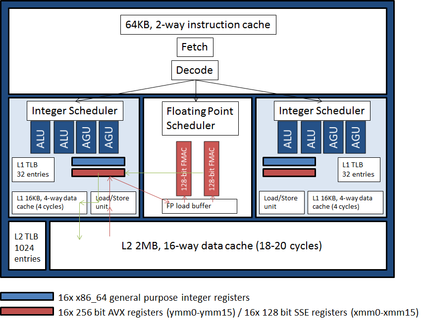
Figure 2. Detailed view of an Interlagos module. The red and green arrows give an example of the movement of data. Red arrows show some operands being loaded into registers from L2 cache before being dispatched into the FMAC (floating point multiply/accumulate) execution units with the result (green arrows) being written back into a register before being placed in L1 and L2 cache (L1 is a write-through cache).

Each die consists of 4 modules which share 6MB L3 data cache (plus 2MB which is reserved in hardware for maintaining cache coherency amongst the dies within a node) and is further connected directly to 8GB of memory. This is illustrated in Figure 3.

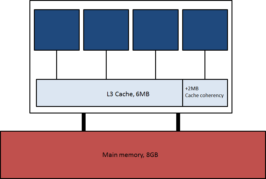
Figure 3. An Interlagos die. Each blue square represents a module, containing 2 cores.

As in phase 2b the HT links are organised in a NUMA (Non-Uniform Memory Architecture) topology in which off-die bandwidth is greatest within a chip, less to the counterpart die in the neighbouring chip and less again to the opposite die in the neighbouring chip, in the ratio 3:2:1. This is illustrated by the number of links between dies in Figure 4.

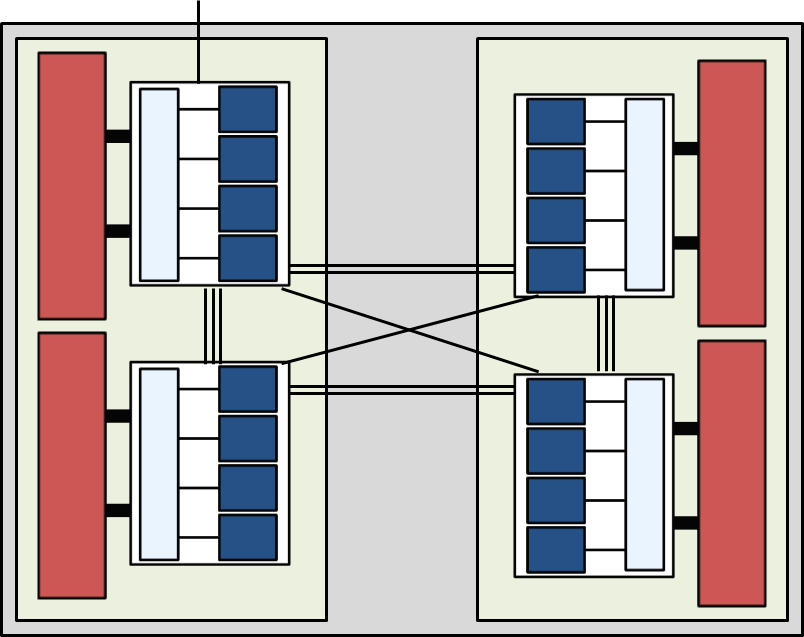
Figure 4. A node (grey) consists of two AMD Interlagos 16-core chips (light green) in the same NUMA topology as in phase 2b, with bandwidth between the dies (white) being in the ratio of 3:2:1 depending on which die data is coming from/going to, as indicated by the number of inter-die connections. There is again a single HT connection off node into the Gemini interconnect.

The Gemini Interconnect

Batch Submission

  #!/bin/bash --login
  #PBS -N My_job
  #PBS -l mppwidth=512
  #PBS -l mppnppn=32
  #PBS -l walltime=00:20:00
  #PBS -j oe
  #PBS -A budget
  
  cd $PBS_O_WORKDIR
  export OMP_NUM_THREADS=1

  aprun -n 512 -N 32 ./my_mpi_executable.x arg1 arg2 > stdout

The following points need bearing in mind:

1. Your job will not share nodes with any other job, thus you will be charged for an entire node of 32 cores even if you actually use fewer than 32.
2. The #PBS directives that appear at the top of a job script tell the job submission system how many compute nodes your job will require.
3. The options given to the aprun command determines the resources your job actually uses.
4. We recommend always setting OMP_NUM_THREADS in your job scripts explicitly because Cray's Lib Sci library is compiled with OpenMP enabled by default.

In order to make things clear, we recommend that mppwidth is always the least upper bound number of processes you intend to use that is a multiple of 32, that mppnppn is always set to 32, and that mppdepth is never used.

Due to the use of many shared resources within an Interlagos module it may make sense to use only a single core per module with dedicated access to the floating point unit, such that half the number of MPI processes may give much better than half the performance. Altering the fully packed job script example above:

  #!/bin/bash --login
  #PBS -N My_job
  #PBS -l mppwidth=512
  #PBS -l mppnppn=32
  #PBS -l walltime=00:20:00
  #PBS -j oe
  #PBS -A budget
  
  cd $PBS_O_WORKDIR
  export OMP_NUM_THREADS=1

  aprun -n 256 -N 16 -d 2 -S 4 ./my_mpi_executable.x arg1 arg2 > stdout

This job script requests the same number of nodes (ceiling(mppwidth/mppnppn) = 512/32 = 16), and thus reserves 512 cores. However, it only actually uses 256 cores for MPI processes (aprun -n 256) and places 16, rather than 32, processes per node (aprun -n 256 -N 16). Finally, the default placement of processes within a node is to assign to cores sequentially, meaning that processes will share modules. In order to spread the processes out so that one process per module is placed, we reserve the second core per module for multithreading and place 4 processes per die (aprun -n 256 -N 16 -d 2 -S 4), even though we have not actually enabled multithreading in this example.

In order to enable multithreading in this example (e.g. if my_mpi_executable.x had been linked to a multithreaded version of the Cray libsci library via -lsci_cray_mp on the link line if using the Cray compiler, -lsci_gnu_mp if using the GNU compiler) then the idle core per module could be utilized for BLAS calls simply by adding export OMP_NUM_THREADS=2 in the job script above. This would then become a hybrid (or mixed mode) job script. Note that by turning on multithreading we may in fact undo the improvement in efficiency brought about by using only a single process or thread per module because we are re-introducing some contention on shared resources.

If your application makes extensive use of OpenMP or multithreaded libraries throughout then you may want more threads per MPI process. The natural configuration for a hybrid job is to use 8 threads per process. For example:

  #!/bin/bash --login
  #PBS -N My_job
  #PBS -l mppwidth=512
  #PBS -l mppnppn=32
  #PBS -l walltime=00:20:00
  #PBS -j oe
  #PBS -A budget
  
  cd $PBS_O_WORKDIR
  export OMP_NUM_THREADS=8

  aprun -n 64 -N 4 -d 8 -S 1 ./my_mpi_executable.x arg1 arg2 > stdout

Phase 3 Checklist

• Have you recompiled your code, linking to the latest libraries?
• Have you investigated a selection of different ways of running your jobs?
• Have you updated your batch scripts with the appropriate PBS and aprun flags?
• Have you benchmarked your jobs and compared performance with phase 2b?
• If your jobs are underperforming have you profiled your code and thought about optimization?

If you would like help with any of the topics discussed in this guide, particularly if you think you may be disadvantaged by the phase 3 upgrade, then please contact the NAG CSE team via the helpdesk: support@hector.ac.uk.

The NAG CSE team runs regular training courses on all of the topics discussed above, and more (see the References section). Check the schedule for current courses. If you would like to attend a course not currently scheduled, please [Email address deleted].

References

• The previous good practice guide for phase 2b puts the upgrade into context.
• An in-depth explanation of AMD's Bulldozer architecture.
• A discussion of AVX instructions from the perspective of the Portland compiler team.
• If you would like to learn more about OpenMP, optimising codes for multicore architectures, profiling and optimisation, or parallel IO the NAG CSE service runs regular training courses which are free for anyone eligible to use HECToR (even if you currently don't have an account). Please check the training schedule and get in touch if you would like to arrange training at your institution free of charge.

Fri Aug 2 09:39:36 BST 2013