
Good Practice Guide
HECToR Phase 2B (24-core)
Contents
As of February 2011 the main machine of the HECToR service in phase 2b is a Cray XE6.
The XE6 consists of 1856 24-core nodes, giving 44,544 cores
in total, increasing the theoretical peak performance and memory footprint from around 200TF and 45TB
in phase 2a to over 370TF and 59TB in phase 2b.
The phase2a XT4 is still currently operational, although this is no longer the contractual service machine.
This guide explains the key differences in software and architecture which will impact the operation and
performance of codes on the XE6 part of the HECToR service.
The section on Architecture below highlights the key changes that will have an effect on
performance. Phase 2b offers nearly double the number of cores compared to phase 2a and is therefore another upgrade
that will favour codes that scale well.
The microarchitecture of the system at the level of a single core is very similar to that of the Barcelona processor
used in phase 2a and therefore the same emphasis should be put on using the 3-level cache hierarchy
effectively and ensuring the use of packed SSE instructions (for more details on these aspects, see the phase 2a guide).
Codes that do not use cache and packed SSE instructions effectively will require some work in order to get the most out
of the new system and are likely to perform poorly if performance issues are not addressed.
The per-core memory statistics show that there will be a decrease in memory size (8GB shared between 6 cores
for the XE6 vs 8GB shared between 4 cores for the XT4), but an increase in memory bandwidth (85.3GB/s across a node vs 12.3GB/s across a node),
which means that memory-access-bound codes may show some benefit, but there may be a need to run larger jobs in order to fit
the same problems in memory. The new architecture also means that much more shared memory is available, 32GB within
a node, which will provide codes that were previously prevented from running on HECToR (due to the previously much smaller
available memory-per-node) with the opportunity to use the XT part of the service for the first time, and also benefit codes that
are able to make effective use of more shared memory.
The new phase 2b system will be less forgiving of codes that perform adequately on the phase 2a system. For example, codes
that scale only to the point that enough processes are used to distribute 2GB of memory per core in phase 2a are likely to
perform very poorly when scaled to higher numbers of processes in order to distribute 1.3GB of memory per core in phase 2b.
Set aside some time to benchmark your code on the new system and compare the results with those
from the phase 2a quad core setup. See the
Good Practice Guide for Performance Measurement for tips on how to benchmark your code.
The upgrade is also a good time to check that you are using libraries wherever possible. This is important
in order to make your life as a developer easier and take advantage of the dedicated
effort put into solving a specific problem efficiently. Make sure you are using the most up to date
versions.
For example, FFTW 3 is designed to make use of packed SSE instructions, whereas FFTW 2 is not,
so it may be worth the effort to switch to the new interface. Remember too that vendor-tuned libraries
(ACML and libsci) are likely to provide the most efficient routines in most cases.
One of the most important aspects of achieving high performance with the AMD Magny Cours processors, which make up the XE6, is utilising
packed SSE instructions, and it is the compiler's job to generate these for you. In order to make
sure that packed SSE instructions are being used for the key computational regions of your code use the compiler options
-Minfo for the PGI compiler (-Mneginfo to see what is not vectorized, which may be more important)
and -LNO:simd_verbose=ON for the Pathscale compiler.
See the Good Practice Guide for Serial Code Optimisation for information about
compiler optimisation flags.
If compiler optimisation fails to improve performance significantly, the next step is code optimisation.
Use CrayPAT to profile your code and understand the performance
bottlenecks. It will be more important to use techniques for effective cache management
such as loop reordering, cache blocking and prefetching. Also, remember that single precision floating point
operations can be carried out at twice the rate of those in double precision, so use double precision
reals only where required. See the Good Practice Guide for Serial Code Optimisation
for more information about code optimisation.
Hybrid MPI-OpenMP programming may be an option to consider if each process in your code currently
contains significant computational sections (e.g. loops) that may be more finely parallelised.
Hybrid codes make use of MPI for inter-processor communication and OpenMP for intra-process communication,
so that some or all cores within a node use multithreaded shared memory parallelism.
The advantage of this approach is that the threads within a process can share much of the same data
structures, thus providing more scope for cache optimisation and also reducing off-node traffic.
The natural way to configure a hybrid job under the architecture
of an XE6 node is to use 4 MPI processes per node, and within each node use 6 OpenMP threads running on the same
die, thus giving uniform memory access to the threads in a process.
It is possible to use all 24 cores within a node for shared memory OpenMP threads, but this may not be desirable,
depending on how your code accesses memory. See the architecture, batch script
and appendix sections for more information on these aspects of running jobs.
Finally, the need to scale to higher numbers of processes means that if your code
performs well at the node level, the limiting factor will become sequential activities such as IO.
Such activities may have had a tolerable impact on performance in the past, but in order to scale further, phase 2b may be the
time to parallelise these regions too. For the specific case of IO, see the parallel IO section of the
Good Practice Guide for IO.
A single node
An XE6 node consists of 24 cores sharing a total of 32 GB of memory accessible through a
NUMA
(Non-Uniform Memory Architecture) design. The 24 cores are packaged as 2 AMD Opteron 6172 2.1GHz processors,
code-named "Magny-Cours".
It is necessary to look at the architecture of a Magny-Cours processor in order to understand the NUMA nature
of an XE6 node.
A Magny-Cours processor is an example of a Directly Connected
Multi Chip Module processor.
Multi Chip Module (MCM) means that the processor is
essentially two hex-core dies (see definition 2) connected
together within the same socket.
Each die has direct access to 8GB memory through 2 memory channels. Access to memory
connected to other dies must be transferred through a
Hyper Transport (HT) link.
Each die has four HT links, which is each
16-bits in width, and one of the links is split into two 8-bit connections.
- One and a half links are connected to the neighbouring die within the Magny-Cours processor, giving a 24-bit HT version 3.1
connection within the processor (38.4GB/s bidirectional bandwidth).
- Within an XE6 node a whole HT 3.1 link connects a die to its counterpart in the neighbouring processor
(i.e. die 0 in processor 0 has a 16-bit connection to die 0 in processor 1, giving 25.6GB/s bidirectional bandwidth).
- Half a HT 3.1 link connects a die to the other, "diagonally opposite", die in the neighbouring processor
(i.e. die 0 in processor 0 has an 8-bit connection to die 1 in processor 1, giving 12.8GB/s bidirectional bandwidth).
- The remaining link is unused in 3 of the 4 dies and in the fourth it is a 16-bit HT version 1 link connected to the interconnect for inter-node
communication and IO, with a bidirectional bandwidth of 6.4GB/s. That only one link is directly connected to the interconnect
gives interesting results for inter-node communication.
Under this architecture, even though each die is directly connected we have an
hierarchy of HT connections and it is this hierarchy which characterises
the NUMA nature of an XE6 node: for a process running on a given core,
accessing memory local to the die belonging to the core is faster than accessing the memory connected to the
neighbouring die, which is faster than accessing the memory connected to the counterpart die in the neighbouring
processor, which is again faster than accessing the memory connected to the diagonally opposite die in the neighbouring
processor. The results of a benchmark test demonstrate the performance differences.
Within a single hex-core die there is 6MB of shared L3 cache, 512KB of dedicated L2 cache, 64KB of dedicated
L1 data cache and 64KB of dedicated L1 instruction cache. Not all of the 6MB of L3 cache will be available
to processes running on the die because around 1MB will be used to support a mechanism called HT Assist
for reducing the amount of Hyper Transport traffic between dies due to maintaining cache coherency. Instead of
constantly probing the caches of other dies, which means communicating via the HT links, a "probe filter" is
maintained in L3 cache, thus effectively improving memory transfer bandwidth and latency between dies.
5MB L3 cache shared between 6 cores represents an increase in the amount of cache available per core compared to
the 2MB L3 cache shared between 4 cores in phase 2a. L1 and L2 cache sizes remain the same. 32GB shared between 24 cores
is a decrease in the amount of main memory per core compared to the 8GB per 4 cores in phase 2a. However, should
users wish to do so, there is the opportunity of running sparsely populated jobs so that more memory is available
per core (up to 32GB if only one core per node is used), which offers more flexibility although at a higher AU cost.
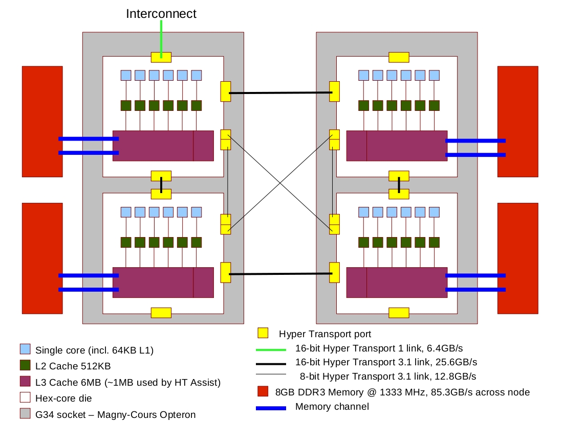
Figure 1: A logical view of the architecture of an XE6 node. Note that there is a connection and a half between
dies in the same socket/Magny-Cours processor.
The Gemini Interconnect
A new interconnect (codenamed 'Gemini') forms a key part of the XE6 system. Compared to the previous SeaStar interconnect this improves the
performance of communication-bound codes and also directly supports in hardware
Partitioned Global Address Space
(PGAS) languages such as Coarray Fortran and UPC, as well as asynchronous one-sided
messaging approaches such as Shmem and one-sided MPI. Prior to the introduction of Gemini the system was an XT6 in which the SeaStar interconnect
represented a serious performance bottleneck for some codes, making optimisations such as using shared memory segments to coalesce messages into a single
off-node communication (as discussed in the Parallel Optimisation good practice guide) and mixed-mode programming crucial for
communications-bound codes; with the introduction of Gemini these optimisations are less crucial, but nonetheless are likely to remain relevant for future
architectures.
There are some important differences between submitting jobs for the XE6 and XT4 that you will need to
understand. If the batch system is used incorrectly, then you may be using more AUs than you realise because a job will always be
charged for an entire compute node of 24 cores even if it actually uses fewer than 24 cores to execute, since
compute nodes are not shared between different jobs.
Pure MPI jobs
Here is an example batch script:
  #!/bin/bash --login
  #PBS -N My_job
  #PBS -l mppwidth=48
  #PBS -l mppnppn=24
  #PBS -l walltime=00:20:00
  #PBS -j oe
  #PBS -A budget

  cd $PBS_O_WORKDIR

  aprun -n 32 -N 16 ./my_mpi_executable.x arg1 arg2 > stdout
Note that we advise against the previous recommended practice of using awk within a batch script to set the values of variables NPROC and NTASKS to match the PBS requested values of mppwidth and mppnppn.
The reason for this is because it is important to make a clear distinction between the
resources requested (i.e. what is specified
in the PBS directives at the top of your job script) and those actually used
(i.e. the values passed to the aprun flags -n, -N, -d, -S).
In the above the job will acutally use 32 cores (aprun -n 32) that span 2 compute nodes (making use of 16 cores in each compute node for load-balancing),
hence mppwidth=2*24=48 requests 48 cores.
The following points need bearing in mind:
-
Your job will not share nodes with any other job, thus you will be charged for an entire node of 24 cores even if you actually use fewer than 24.
-
The #PBS directives that appear at the top of a job script tell the job submission system how many compute nodes your job will require.
-
The options given to the aprun command determines the resources your job actually uses.
In order to make things clear, we recommend that mppwidth is always the least upper bound number of processes you intend to use that is a multiple of 24, that mppnppn is always set to 24, and that mppdepth is never used.
Hybrid MPI/OpenMP jobs
Here is an example batch script:
  #!/bin/bash --login
  #PBS -N My_job
  #PBS -l mppwidth=96
  #PBS -l mppnppn=24
  #PBS -l walltime=00:20:00
  #PBS -j oe
  #PBS -A budget

  cd $PBS_O_WORKDIR
  export OMP_NUM_THREADS=6
  # This variable should be set to allow the ALPS and the OS scheduler to
  # assign the task affinity rather than the compiler. If this is not set
  # they you may see a large negative effect on performance.
  export PSC_OMP_AFFINITY=FALSE

  aprun -n 15 -N 4 -d 6 -S 1 ./my_mpi_executable.x arg1 arg2 > stdout
This last example gives the "natural" configuration for a hybrid job discussed above: on each node we are placing 4 MPI processes, one on
each die, and each process may fork 6 threads to run on the same die. This example uses ceiling(15/4) = 4 compute nodes.
Note that the -S aprun flag is a new one, which defines how many processes to put on each die in order to allow an even distribution for sparsely populated jobs (i.e. jobs in which fewer than 24 processes are used per node). By default processes are placed sequentially within a node, that is die 0 is filled first (top left in Figure 1), then die 1 (bottom left) then die 2 (top right) and then die 3 (bottom right). Note, if you are using a multi-threaded version of libsci 10.4.1, set GOTO_NUM_THREADS rather than OMP_NUM_THREADS in your job script.
We recommend users base their job scripts on either of the above examples, unless there is a good reason not to.
For example, running jobs sparsely populated within a node in order to utilise more memory per process, in which case
you should consult the user guide
and aprun man page or contact the helpdesk for assistance.
CSE Assistance
If you would like to explore how to take advantage of the potential performance increase
available in phase 2b, or would like dedicated help and advice on benchmarking, profiling or improving your code, please get in touch
with the NAG CSE team:
hector-cse@nag.co.uk.
The CSE team run regular training courses on the topics discussed above, and more (see the References section).
Check the schedule for current courses. If you would
like to attend a course not currently scheduled, please contact us.
Appendix: some micro-benchmarking results
Mon Jun 14 15:51:36 BST 2010