Good Practice Guide

Serial code optimisation

Introduction
Compilers and libraries
Writing optimised code
Example
References

Introduction

This guide presents the main features of serial optimisation for computationally intensive codes with a focus on the HECToR computing resources. From a user's point of view two main avenues can be followed when trying to optimise an application:

Optimisations that DO NOT involve modifying the source code (modification may not be desirable): optimisation consists of searching for the best compiler, set of flags and libraries.
Optimisations that DO involve modifying the source code: in the first instance the programmer must evaluate if a new algorithm is necessary, followed by writing or rewriting optimised code. The simplest way to gain performance is to use performance-tuned libraries for numerically intensive sections. If this is not possible the programmer should write the code using techniques that help the compiler to generate a fast executable.

According to the above choices this guide presents optimisation as a problem of compiler and library selection in the next section, followed by a presentation of the key factors that must be considered when writing numerically intensive code in the subsequent sections.

Compilers and Libraries

Compilers

Modern compilers offer in general very good optimisations using code transformations that attempt to reduce the number of instructions and to maximise the computational throughput (i.e. number of operation per CPU clock step). The user guides of each compiler installed on HECToR , Ref [1], present detailed information on this subject, here we present just a short summary.

The available optimisations can be classified broadly as follows:

local optimisation in logical blocks: algebraic identity removal, constant folding, common sub-expression elimination, redundant load and store elimination, scheduling, etc;
global optimisation: analyses an entire program unit and can do constant propagation, copy propagation, dead store elimination, induction variable elimination, invariant code motion;
loop optimisation: unrolling, vectorisation;
inter-procedural analysis: allows use of information across the function call boundaries for extra optimisation;
function inlining: replaces a function call with its body, if useful.

Not all optimisation transformations always lead to faster code but each compiler has a set of generic optimisation flags that improve performance significantly in almost all cases. These generic flags are combinations of low level switches that can be adapted further for a specific application. Two more kinds of flags are useful during optimisation process: (i) the documentation flags that can be used to ask a compiler for more information about optimisation flags and (ii) the info flags that provide information on the success or failure of attempted optimisation on the source code.

Below we describe briefly for each compiler the generic optimisation flags together with the descriptive and info flags. User guides and man pages must be studied for complete and up to date information.

Cray

The general levels of optimisations -O1, -O2, -O3 include varying degrees of vectorisation, scalar optimisations and inlining, default level is -O2.
-e o displays the optimization options used during compilation
-rm generates a .lst file for each source file with annotated source code and messages on successful and failed optimisations.

PGI

-fast Mipa=fast chooses generally optimal flags for the target platform. Use pgf90 -help -fast to see the low level flags.
For C++ code add -Minline=level:10 --noexceptions and consider -Msafeptr flag and the finer-grained #pragma safeptr directive when you are confident that pointers do not share storage.
Other optimisation flags most likely to improve performance are: -O1 to -O4, -Mpfi, -Mpfo, -Minline, -Munroll, -Mvect
-help can be used in combination with another option to see its description.
-help=opt prints help for optimization command-line options.
-Minfo -Mneginfo generates an annotated source code with information about successful or failed optimisation transformations.

GNU

-O1, -O2, -O3, -Ofast provide incremental sets of optimisation assumed to be useful in general. Specific optimisation can be turn on or off with option of the form -fflag -fno-flag.
-Os optimises for executable size.
A description of the low level flags enabled by level n={1,2,3} can be obtain with the following command: gcc -c -Q -O{n} --help=optimizer.
-ftree-vectorizer-verbose=n, n=0-9, generates information on the the vectorised loops

On HECToR the desired compiler (vendor and version) should be selected via the module programing environment.

For many complex scientific applications performance varies significantly for executable binaries generated with different compilers. Information about the best suited compiler for a given application can be found from the user community but it is good practice to test this information as architectures and compilers evolve at a relatively high pace on HPC systems.

The HECToR website provides a compiler performance comparison page for a set of applications used on HECToR which contains also examples of optimisation flags combination used for the respective applications. The results show that performance can be increased up to 20% just by selecting the right compiler with the right combination of flags.

Before concluding this section is worth mentioning that the optimisation level might need to be decreased for files on which compilation crashes, or if the application crashes or produces incorrect results. To test the numerical accuracy between two architectures, non-optimised executables should be used if possible.

Libraries

Using libraries for standard numerical operations avoids programming errors and conserves code performance across platforms. Ideally all numerical intensive task should be delegate to libraries leading to a code layout similar to Fig 1.

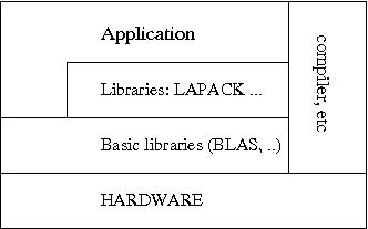
Fig. 1: Layers of library calls ensure portable numerical performance.

For example, the following code section

	  DO I = 1, N 
	  Y(I) = 0.0D0 
	  DO J = 1, M 
	  Y(I) = Y(I) + 2.0D0*A(J,I)*X(J) 
	  END DO 
	  END DO

is equivalent to a BLAS call

	  CALL DGEMV('T',M,N,2.0D0,A,LDA,X,1,0.0D0,Y,1)

On HECToR several suites of libraries are available, Cray's Lib Sci is the default library; ACML and NAG libraries are also installed on HECToR (accessible via module environment). They provide the standard linear algebra packages (BLAS, LAPACK), fast Fourier transform, random number generators and much more. Up to date information on components and versions of each library can be found in the User Guide and man pages. If the code spends a significant amount of time in some library routines it is good practice to check if the selected vendor and version of the library is the one best suited for the application. As mentioned above, user or developer community wisdom is the way to avoid blind search.

Writing optimised code

Background

For the remainder of this guide we focus on some of the core optimisation techniques for numerically intensive codes. In general two main factors determine the speed of a computation: (i) the algorithm efficiency, i.e. the number of steps it needs to complete a computation for a given input, and (ii) how well the executable exploits processor architecture.

Accordingly, the first step for a fast implementation is to select the best algorithm considering the constrains and the range of values for the parameters defining the problem. As scientific applications tend to be applied to larger problems in time (large in the sense of number of particles, grid points, etc.) it is very important to use algorithms that have good scaling properties for the parameters of interest. On the other hand the programmer should not overkill the problem. Complicated algorithms are harder to maintain and error prone. Even if a new algorithm is asymptotically faster one has to check if the operating regime of interest is included in the domain of parameters in which the new algorithm performs better (e.g. there are algorithms which asymptotically are faster but they don't bring any benefit in the intermediate regime).

The second step is to write the source code in a way that makes efficient use of processor capabilities. A short technical digression is useful here in order to make clear why certain code patterns are desirable for performance.

Instruction and data parallelism optimisation

Modern processors have two main hardware features designed for parallel processing of large amounts of floating point instruction and data:

pipelines:: which decomposes the floating point instruction in stages. In this way multiple instruction can pass through the pipeline at the same moment of time, if they are independent. In an ideal situation each pipeline can produce a floating point result per clock step even if each floating point instruction takes several clock step to complete.
vector registers:: a pipeline can operate on a set of floating point data (single or double precision) using wide registers (128 or 256 bits). Execution speed is improved by combining an addition and a multiplication into a single processor instruction, the so called fused multiply-add.

The architecture details of the processor used on phase 3 of HECToR and its peak performance are presented in this document .

The programmer should try to use constructs that expose the instruction-level parallelism to the compiler but avoiding heavy code containing simple optimisations that a modern compiler can do, see Ref [2].
In numerically intensive kernels the following rules help optimisation in general:

avoid function calls, test statement, jumps, ambiguous pointers;
avoid unnecessary data dependencies, complicated common sub-expressions;
loops with a low trip counts or not enough computation in the body should be unrolled;
for vectorisation memory must be accessed with stride 1, and for nested loops the longest loop count should be innermost with stride 1.

A good starting point for optimisation work is to compile the code using info flags which will generate a report with the tried optimisation and possible causes for not applying some optimisation transformations.

Cache optimisation

Although HECToR's processor can perform more than one floating point operation per clock step with data from registers the access time to main memory is of the order of hundreds of clock steps. The technological solution for this disparity is to use a hierarchy of smaller cache memories that have shorter access times. In the current configuration HECToR processors have one individual cache level per core, a second level shared by two cores (the so-called module) and a third level shared across 8 cores (the so-called die). The cache helps because if a memory address is used by the processor at a given instant there is in general a high probability to use the address again, or one in its close vicinity, after a short time interval. Therefore, performance can be improved further by seeking actively to access the memory in local patterns which allows use of the data already in cache as many times as possible.

There are two types of locality:

temporal: refers to multiple usage of the same data item in a short period of time while the data resides in the cache memory. Temporal locality can be achieved in short loops free of function calls or branching statements;
spatial: refers to usage of data located in a block of consecutive addresses. Since a load instruction for one address brings in the cache memory data located a block of consecutive addresses in the main memory (called a cache line), performance is gained if data from neighbouring addresses are used in subsequent operations while that data still resides in cache.

A simple example that shows the importance of spatial locality is the order of the nested loops over matrix elements. If the matrix does not fit in first level cache memory the computation is significantly faster if the inner loop goes over the first index in Fortran or over the second index in C, thus accessing neighbouring elements in memory.

We mention briefly two more technical aspects which are important in memory optimisation.

For performance purposes each memory address is mapped only to a number of predetermined cache lines (2,16,48 lines for for L1, L2, L3 cache levels respectively on HECToR phase 3). This is called n-way set associativity and it raises the possibility of pathological cases (particularly in the 2-way case) in which two array variables involved in the same operation use the same cache line. In such cases a significant performance loss occurs because the cache line must be refilled twice for each array element operation. A solution to this problem is to pad the array with extra memory elements and to avoid array sizes in powers of 2.
Applications use a virtual space of addresses that are translated by the operating system into physical memory addresses. Information about recently used physical addresses are held in special cache named the translation lookaside buffer (TLB). If a physical address cannot be found in the TLB then the main memory must be accessed for extra information with a significant performance penalty. From an application's perspective TLB misses occur typically in sections of code that work through array indices with large strides.

Performance analysis tools are helpful in spotting cache utilisation problems.

Memory management and OOP

Modern programing languages offer dynamic memory allocation which allows for greater code flexibility. However memory allocation/deallocation are time consuming operations and they must be avoided in subroutines or functions that are called frequently. The high-water technique is a way to reduce the need for these expensive calls, see e.g. Ref [2].

If the code is written in C++ a couple of specific points should be considered for optimisation: excessive time spent in object creation and destruction, function call overhead, pointer aliasing. This online book, Ref [5], presents details of C++ optimisation specific issues and also an overview on general aspects of optimisation.

Optimising the optimisation process

Mastering the intricacies of optimisation techniques needs dedicated study from books, e.g. Refs [2, 3, 4], training courses and lots of practice. A systematic approach is very useful in this kind of work because a fair amount of time is typically spent in the processes with the exploration of the code variants. Before starting it is very important to estimate the possible performance gain from a performance analysis which can identify the code sectors worth an optimisation effort and what sort of optimisation is needed (e.g. memory access vs computation). During the process each new version of the code should be compiled with the info flags switched on and its performance recorded.
For clarity and debugging it is advisable to keep at hand the original version of the code.

Example

The main points discussed in this guide are illustrated in Fig 2 which presents the computation speed for a dot product operation on two arrays against their size. The three runs correspond to executables compiled with different set of optimisation flags, of which one includes vectorisation. Notice the speed doubling in single precision with respect to the double precision case at around array size 1000 for the executable compiled with vectorisation flag. This is due to the fact that twice as many operands are packed in the vector registers if single precision data are used. The cache effect are visible as steps in performance as the size of the data array increases. Using single precision data allows for larger arrays to be processed faster than compared with their double precision counterpart.

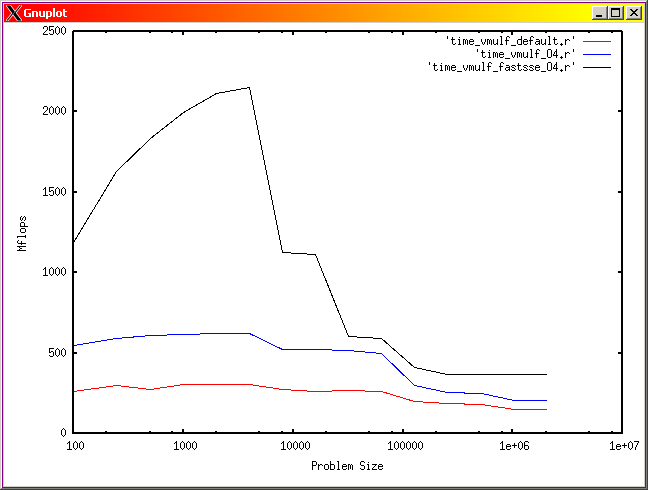
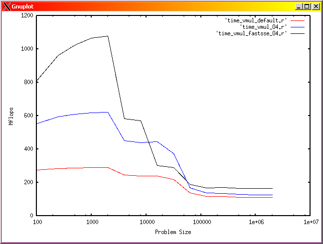
Fig. 2: Computation intensity for a dot product operation function of the array size in single precision (left), and double precision (right). Red line is for an executable compiled with default optimisation, blue is for an executable compiled with -O4 flag and black line correspond to an executable compiled with a vectorisation flag.

References

Cray Fortran Reference Manual, PGI User Guide, GCC optimisation options , AMD compiler options quick reference guide.
Suely Oliveira & David Stewart, Writing Scientific Software, A guide to good style, Cambridge University Press, 2006.
Stefan Goedeker, Adolfy Hoisie, Performance optimization of numerically intensive codes, SIAM, 2001.
Kevin Dowd, Charles Severance, High Performance Computing, O'Reilly, 1998.
Optimising software in C++, by Agner Fog: http://www.agner.org/optimize/optimizing_cpp.pdf