$\vec{k}$-point Parallelisation

Figure 9: Interaction range of primary set atom $i$ with its neighbour $j$ and the corresponding periodic images $j'$. All $j$ and $j'$ are in he neighbour list of $i$.

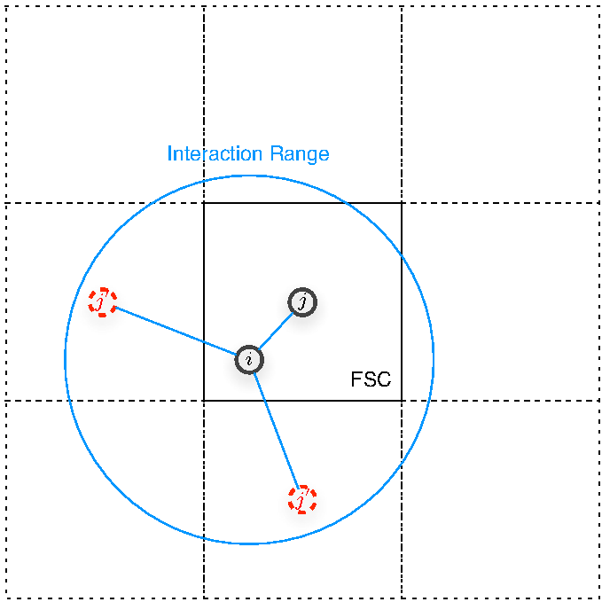The CONQUEST implementation of matrices do not regard any system (bulk or otherwise) to have periodic boundary conditions, instead the code treats any location in real space as it is[5]. The cell from user input is regarded as the Fundamental Simulation Cell (FSC), and the FSC is repeated in all lattice directions so that all atoms taking part of interaction with that inside the FSC are taken account of (see figure 9). All quantum-mechanical operators are represented by matrices using support functions (which for the purpose of this report may be regarded as a set of basis functions upon which we have our matrix representation). For details on the meaning of support functions, how these are formed from the (actual) basis--which can either be Pseudo-Atomic Orbitals (PAOs) or B-Spline functions--and how are the quantum mechanical quantities represented by these support functions, please refer to [4,5].

Figure 10: CONQUEST matrix storage format. Each block in the diagram corresponds to $(i,j)$th atom block with dimension $N^i_{\text {sf}} \times N^j_{\text {sf}}$, where $N^{i/j}_{\text {sf}}$ is the number of support functions for atom $i$ or $j$ respectively. $n_{\text {part}}$ is the partition index local to each processing-node.

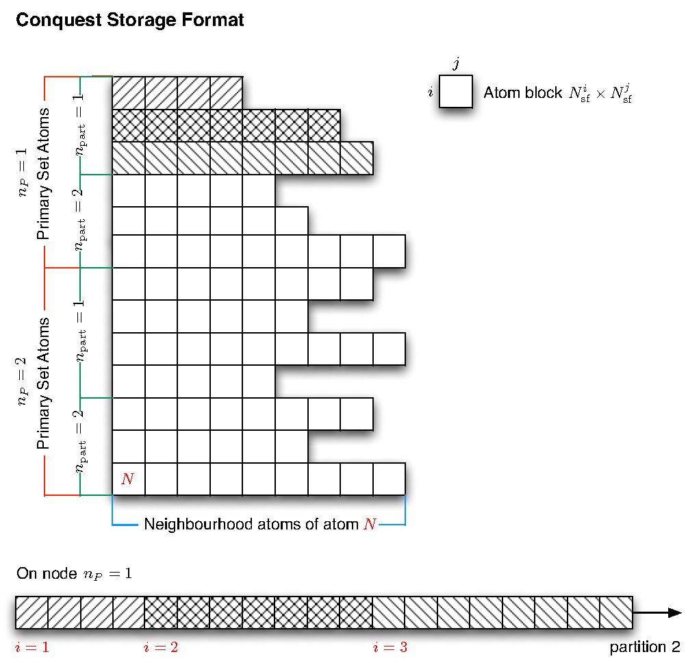The CONQUEST method of storing matrices of the form

$$A_{i\alpha,n\beta} = \int\D^3\vec{r} \phi_{i\alpha}(\vec{r} - \vec{R}_i) \hat{A} \phi_{n\beta}(\vec{r} - \vec{R}_j)$$ (8)

is illustrated in figure 10. The atoms in the FSC are divided among the processors and the set of FSC atoms responsible by each processor is called a primary set. To give CONQUEST more flexibility in data transfer space is divided into many partitions and atoms contained in a partitioned space are regarded as to belong to the that particular partition. Matrix elements corresponding to the same partition are stored together in continuous piece of memory, and data transfer are normally done partition by partition. Given different matrices (operators) the interaction ranges between atoms differ, a halo atom of a given matrix (range) type is then defined to be any atom that is within the interaction range of the any atoms of the primary set. A set halo atoms corresponds to the union of the set of neighbours (neighbour-lists) of the primary set atoms. A halo partition of a given interaction range is then any partition that contains at least one halo atom. A halo is then defined to be the collection of all halo partitions corresponding to a given range. And finally a covering set of a given processor is defined as the minimum orthorhombic cell that contains the largest (one corresponding do the longest interaction range) halo. In $A_{i\alpha,n\beta}$ defined in equation (14), on each node $i$ indexes the primary set atoms responsible by the processor, and $n$ indexes the atoms in the covering set. Moreover, not all terms with a given $n$ is stored, only those actually in the neighbour-list of each primary set atom $i$ is stored piece-wise in a row-major format (see figure 10).

To update the electron density CONQUEST solves the generalised eigen-value problem

$$\sum_{j\beta} {\tilde{H}}\ind{^{\vec{k}}_{i\alpha,j\beta}} ... ...^{\vec{k}}_{i\alpha,j\beta}} c\ind{^{\vec{k}}^{j\beta}_{n}}$$ (9)

where indices $i$, $j$ index the atoms in the FSC, and $\alpha$, $\beta$ index the support functions associated to the corresponding atom. ${\tilde{H}}\ind{^{\vec{k}}_{i\alpha,j\beta}}$ corresponds to the matrix representation of the Hamiltonian operator under periodic boundary conditions:

$${\tilde{H}}\ind{^{\vec{k}}_{i\alpha,j\beta}} = \int\D^3\vec... ...\hat{H} \tilde{\phi}^{\vec{k}}_{j\beta}(\vec{r} - \vec{R}_j)$$ (10)

where the Bloch sums of support functions are defined as $$\tilde{\phi}^{\vec{k}}_{i\alpha} = \frac{1}{\sqrt{N}} \sum_... ...}\cdot(\vec{R}_i + \vec{a})} \phi_{i\alpha}(\vec{r} - \vec{R}_i)$$ and $N$ is normalisation factor, $\vec{a}$ is any linear combination of integer multiples of the lattice constants¹, and $\phi_{i\alpha}(\vec{r} - \vec{R}_i)$ is the $\alpha$-th CONQUEST support function corresponding to atom $i$. All atoms which are periodic images of $i$ share the same support function--i.e. $\phi_{i\alpha}(\vec{r} - \vec{R}_i) = \phi_{i'\alpha}(\vec{r} - \vec{R}_{i'})$ if $\vec{R}_{i'} = \vec{R}_{i} + \vec{a}$. $\tilde{S}\ind{^{\vec{k}}_{i\alpha,j\beta}}$ denotes the overlap matrix under periodic boundary conditions

$$\tilde{S}\ind{^{\vec{k}}_{i\alpha,j\beta}} = \int\D^3\vec{r... ...c{R}_i) \tilde{\phi}^{\vec{k}}_{j\beta}(\vec{r} - \vec{R}_j)$$ (11)

And finally $c\ind{^{\vec{k}}^{i\alpha}_n}$ are the coefficients of the eigenvectors spanned by the Bloch sums of support functions $$\psi^{\vec{k}}_n(\vec{r}) = \sum_{i\alpha} c\ind{^{\vec{k}}^{i\alpha}_n} \tilde{\phi}^{\vec{k}}_{i\alpha}(\vec{r} - \vec{R}_i)$$

It can be shown[3] that the hermitian matrices $\tilde{A}\ind{^{\vec{k}}_{i\alpha,j\beta}}$ such as $\tilde{H}\ind{^{\vec{k}}_{i\alpha,j\beta}}$ and $\tilde{S}\ind{^{\vec{k}}_{i\alpha,j\beta}}$ defined in equation (16) and (17) can be calculated from the native CONQUEST matrices using the relationship

$$\tilde{A}\ind{^{\vec{k}}_{i\alpha,j\beta}} = \sum_{j'} e^{i\vec{k}\cdot(\vec{R}_{j'} - \vec{R}_i)} H_{i\alpha,j'\beta}$$ (12)

where $j'$ indexes the atoms in the covering set which is a periodic image of primary set atom $j$, that is $\vec{R}_{j'} = \vec{R}_j + \vec{a}$ for any $\vec{a}$ being a sum of integer multiples of the lattice vectors.

A call to ScaLAPACK subroutine pzhegvx is made to obtain the set of eigenvalues (the band structure) $\epsilon_n(\vec{k})$ which are used to calculate the Fermi-energy and occupation function (this is discussed briefly in section 3). Once this is done another call to pzhegvx is made to get the eigenvectors for each $\vec{k}$ point, the new electronic density can than be calculated using formula[3]

$$K^{i\alpha,j'\beta} = \sum_{\vec{k}} \sum_{n} f_n c\ind{^{... ...{k}}^{j\beta}_n} e^{i\vec{k}\cdot(\vec{R}_{j'} - \vec{R}_i)}$$ (13)

where again, atoms $j'$ corresponds to the periodic images of the primary set atom $j$ and $\vec{R}_{j'} = \vec{R}_j + \vec{a}$. So $K^{i\alpha,j'\beta}$ again is a matrix with $j'$ extending over the entire covering set, and is a matrix that can be stored in native CONQUEST format. Note that there are two calls to pzhegvx because we cannot calculate the density without knowing the occupation function first, but on the other hand since the band structure needs eigenvalues calculated for all $\vec{k}$ if we are going to make only one call to pzhegvx all eigenvectors are then need to be stored. By calling pzhegvx twice we can save significant memory by simply accumulating the eigenvectors into the density matrix. It was found² also that the call to pzhegvx for only calculating eigenvalues is only about 10% the cost of the full call that also calculates the eigenvectors.

The original CONQUEST implementation solves equation (15) one $\vec{k}$ point at a time. And the matrices $H_{i\alpha,n\beta}$ and $S_{i\alpha,n\beta}$ are then mapped onto new matrices $\tilde{H}\ind{^{\vec{k}}_{i\alpha,j\beta}}$ and $\tilde{S}\ind{^{\vec{k}}_{i\alpha,j\beta}}$ distributed across all available processors arranged in a BLACS processor grid according to ScaLAPACK cyclic block format. The calculated eigenvectors from ScaLAPACK for each $\vec{k}$ are then transfered from ScaLAPACK data format and accumulated into $K^{i\alpha,j'\beta}$ stored across the processors in CONQUEST format, and the self-consistent calculation carries on from there.

We note that calculations involved for solving eigenvectors for different $\vec{k}$ are independent from each other. If we could add a degree of freedom of allowing subgroups of processors working on different $\vec{k}$ then it would allow us to choose better optimised parameters for the ScaLAPACK calculations. For matrices of a given size there is an optimal number of processors that should be allowed to work on it, and too many processors means inefficient communications taking over. Hence parallelising calculation in $\vec{k}$ would in theory allow one to use more processors more efficiently by having groups of optimal number of processors working for each ScaLAPACK subroutine call. Since for metallic calculations, te number of $\vec{k}$ points required are in the order of 1000s, this is a real degree of freedom we can exploit, especially for calculations running on HPC systems such as HECToR.