Next: Test Results Up: -point Parallelisation Previous: -point Parallelisation Contents
We introduced a new user definable parameter ![]() , denoting the
number of processor groups each responsible for different set of
, denoting the
number of processor groups each responsible for different set of
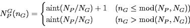
![]() points. We want to allocate a set of
points. We want to allocate a set of
![]() points to each process group
points to each process group ![]() (
(
![]() ), and then
the
), and then
the ![]() processing-nodes inside each group will work on the
processing-nodes inside each group will work on the
![]() points. The cyclic allocation technique is
the most efficient in terms of evenly distributing the work-load. So
that the process-group indices
points. The cyclic allocation technique is
the most efficient in terms of evenly distributing the work-load. So
that the process-group indices ![]() relates to processing-node
indices
relates to processing-node
indices ![]() and
and ![]() -point indices as
-point indices as
| (14) |
 and similarly
We introduced arrays
![]() and
and
![]() to keep track of
which processors and
to keep track of
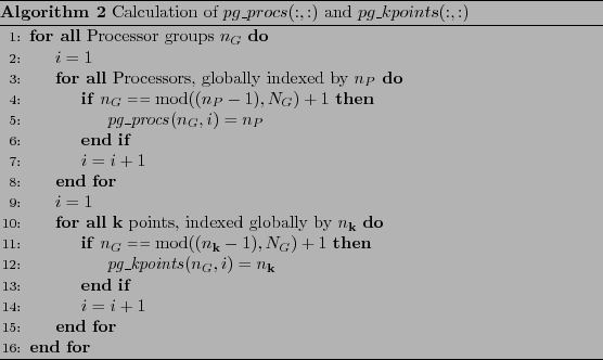
which processors and ![]() points are allocated to which processor
groups. These arrays can be worked out following the steps given in
algorithm 2. Note however that the algorithm is order
points are allocated to which processor
groups. These arrays can be worked out following the steps given in
algorithm 2. Note however that the algorithm is order
![]() (where
(where ![]() is total number of processors), because the same
algorithm is repeated on every processor. However the calculations are
simple and one only has to do it once at the beginning of the
calculation; further more no communication is needed between the
processors.
is total number of processors), because the same
algorithm is repeated on every processor. However the calculations are
simple and one only has to do it once at the beginning of the
calculation; further more no communication is needed between the
processors.
The goal is to define a mapping between the ScaLAPACK block cyclic
format distributed over a processor grid consisting of only a subset
of processors for a given ![]() point and the native
CONQUEST format that distributes the rows of the matrices
into primary set atoms and partitions across the entire set of
processors. In the original CONQUEST implementation, to aid
the mapping a reference matrix format is introduced. This is the
format for the matrices
point and the native
CONQUEST format that distributes the rows of the matrices
into primary set atoms and partitions across the entire set of
processors. In the original CONQUEST implementation, to aid
the mapping a reference matrix format is introduced. This is the
format for the matrices
![]() and
and
![]() which has the same
form as if one writes them down on for calculations on paper. The
reference format matrices are never physically stored. Also in the
original implementation by noticing the fact that the order of atoms
in a calculation can be arbitrary, the atomic ordering of the rows of
the ScaLAPACK format is chosen to be the same as that of the
native CONQUEST format. In other words the atomic ordering
(index
which has the same
form as if one writes them down on for calculations on paper. The
reference format matrices are never physically stored. Also in the
original implementation by noticing the fact that the order of atoms
in a calculation can be arbitrary, the atomic ordering of the rows of
the ScaLAPACK format is chosen to be the same as that of the
native CONQUEST format. In other words the atomic ordering
(index ![]() ) of the ScaLAPACK matrices
) of the ScaLAPACK matrices
![]() and
and
![]() is chosen to be the same
as the ordering of
is chosen to be the same
as the ordering of ![]() in matrices
in matrices
![]() and
and
![]() stored in CONQUEST format. We have kept
this requirement for the implementation
stored in CONQUEST format. We have kept
this requirement for the implementation ![]() point parallelisation.
point parallelisation.
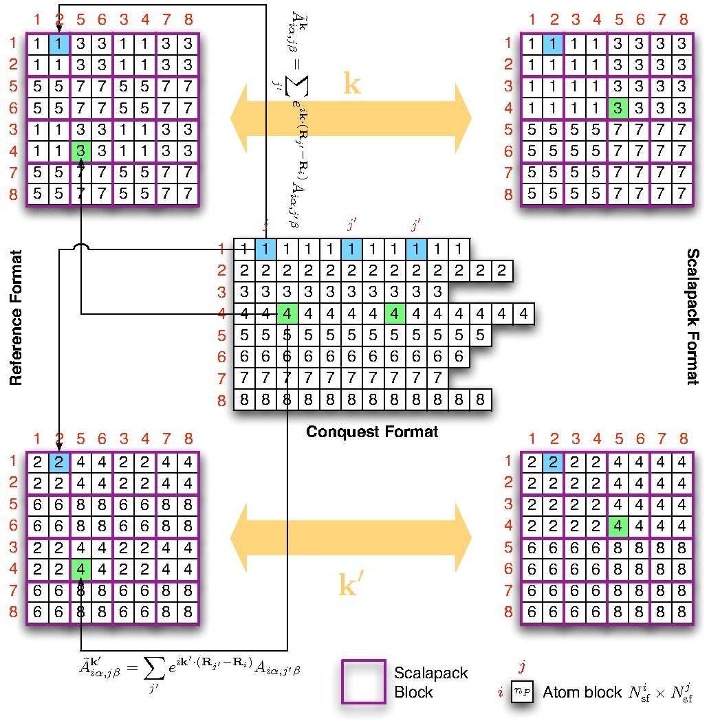 |
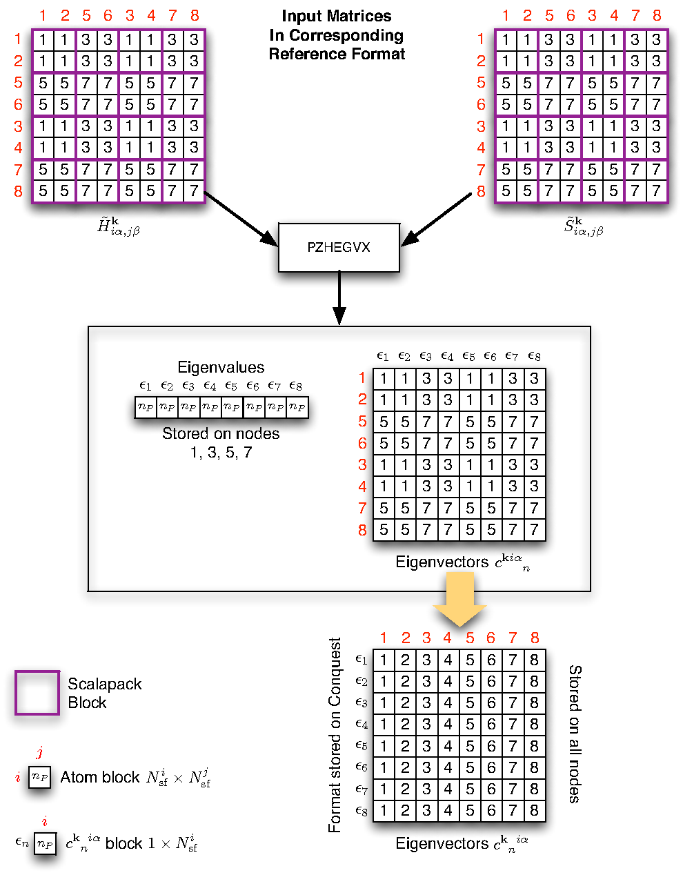
Figure 11 shows the possible mapping of
matrices if there are 8 processors in total and the user have chosen 2
processor groups. The BLACS process grid is assumed to be ![]() and the ScaLAPACK blocks are shown in purple boxes. Due to cyclic
allocation, the first group will have processors 1, 3, 5, 7 (note we are
indexing the processors from 1) and the second group have processors
2, 4, 6, 8. The ScaLAPACK matrix for each group have identical format,
and the matrix elements differ only by the way different
and the ScaLAPACK blocks are shown in purple boxes. Due to cyclic
allocation, the first group will have processors 1, 3, 5, 7 (note we are
indexing the processors from 1) and the second group have processors
2, 4, 6, 8. The ScaLAPACK matrix for each group have identical format,
and the matrix elements differ only by the way different ![]() point is used to generate
point is used to generate
![]() or
or
![]() matrices from the
CONQUEST matrices
matrices from the
CONQUEST matrices
![]() or
or
![]() . The coloured squares in the CONQUEST
matrix shows the periodic images of atoms all belong to the
neighbourhood of a given primary set atom. And their contributions are
summed up according to equation (18) and stored in the
corresponding coloured location in the ScaLAPACK matrix. The numbers
inside the small boxes identify the processor responsible for the data
block.
. The coloured squares in the CONQUEST
matrix shows the periodic images of atoms all belong to the
neighbourhood of a given primary set atom. And their contributions are
summed up according to equation (18) and stored in the
corresponding coloured location in the ScaLAPACK matrix. The numbers
inside the small boxes identify the processor responsible for the data
block.
Since the atomic ordering of rows and columns of the ScaLAPACK is
unchanged from the original implementation, subroutines
find_SC_row_atoms, find_ref_row_atoms and
find_SC_col_atoms of the ScalapackFormat module do not
need to be modified. However the rest of the module as well as the
data transfer modules in module DiagModule do need
modification, to take into account that now the maps to BLACS
processor grid is also dependent on the processor group we are in, and
we have to send one copy of the matrices to each of the ![]() processor
groups.
processor
groups.
To obtain the eigenvectors the ScaLAPACK subroutine pzhegvx
call is made on every processor, with each processor group using a
different set of
![]() and
and
![]() (corresponding to a
different
(corresponding to a
different ![]() ). Upon return from the ScaLAPACK call each
processor group will have a different set of eigenvectors. To build
the density matrix we first map the ScaLAPACK format eigenvectors into
the native CONQUEST format, then accumulate the products of
the eigenvectors one
). Upon return from the ScaLAPACK call each
processor group will have a different set of eigenvectors. To build
the density matrix we first map the ScaLAPACK format eigenvectors into
the native CONQUEST format, then accumulate the products of
the eigenvectors one ![]() point at a time (see equation
(19)). This is preferred because we can then utilise the
pre-existing code for generating density matrix, and only one storage
array for eigenvectors in CONQUEST format is needed on each
processor--as contributions from eigenvectors are accumulated into
the density matrix. Also performance wise the main benefit of
point at a time (see equation
(19)). This is preferred because we can then utilise the
pre-existing code for generating density matrix, and only one storage
array for eigenvectors in CONQUEST format is needed on each
processor--as contributions from eigenvectors are accumulated into
the density matrix. Also performance wise the main benefit of
![]() point parallelisation comes from the freedom it offers for
optimising the ScaLAPACK routine, and building the density matrix is
simply a scalar multiplication and accumulation process hence it is
perfectly efficient to build the density matrix using the parallel
processing format provided by the native CONQUEST approach
(please read [5] for details on how matrix operations
are handled in CONQUEST).
point parallelisation comes from the freedom it offers for
optimising the ScaLAPACK routine, and building the density matrix is
simply a scalar multiplication and accumulation process hence it is
perfectly efficient to build the density matrix using the parallel
processing format provided by the native CONQUEST approach
(please read [5] for details on how matrix operations
are handled in CONQUEST).
Some attention needs to be paid on the mapping from the output
eigenvectors distributed following the ScaLAPACK block-cyclic format
and the BLACS processor grid, to the distribution format for matrices
used by CONQUEST. First important fact to note is that the
ScaLAPACK subroutine pzhegvx returns the eigenvectors in
columns and in the same order as the corresponding eigenvalues
(see Figure 12). On the other hand, in
CONQUEST format for each ![]() each processor is required
to be in charge of a set of atoms in FSC, in other words, a set of
indices
each processor is required
to be in charge of a set of atoms in FSC, in other words, a set of
indices ![]() for the eigenvectors
for the eigenvectors
![]() . And unlike the cases with
conventional matrices in CONQUEST which are stored in
row-major format (i.e. not strictly a matrix in FORTRAN 90 sense), the
eigenvectors are stored as a two-dimensional array. We require
the
. And unlike the cases with
conventional matrices in CONQUEST which are stored in
row-major format (i.e. not strictly a matrix in FORTRAN 90 sense), the
eigenvectors are stored as a two-dimensional array. We require
the
![]() data associated to each
data associated to each ![]() index to stay in one continuous piece of memory, this means a
column-major storage for the eigenvector. In other words in
CONQUEST format the eigenvectors are stored as
index to stay in one continuous piece of memory, this means a
column-major storage for the eigenvector. In other words in
CONQUEST format the eigenvectors are stored as
![]() . That is, the eigenvectors are
stored in rows. The order of eigenvalues also changes from the
ScaLAPACK format, because the CONQUEST format ordering should
be the same as that of the reference format.
. That is, the eigenvectors are
stored in rows. The order of eigenvalues also changes from the
ScaLAPACK format, because the CONQUEST format ordering should
be the same as that of the reference format.
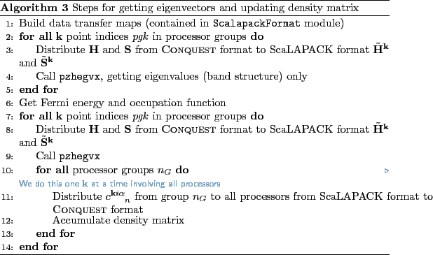
The steps taken to generate the new density is illustrated in
pseudocode algorithm 3. One has to be careful that we do not
step over the limits since it is highly likely that number of
![]() points in each processor group is different, and hence an
points in each processor group is different, and hence an
if statement is required to ensure this.
Lianheng Tong 2011-03-02