Next: Test Results Up: Metal CONQUEST Previous: Test Results Contents
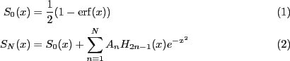
Apart from the effects of charge-sloshing, another main problem
associated with calculations involving metallic systems is that one
must integrate a discontinuous function over the Brillouin zone due to
the partial filling of the band. For numerical integration methods
this requires a very fine reciprocal space mesh (![]() -mesh)
inside the Brillouin zone. One way to rectify this problem is to
approximate the step-function occupation function wit a Fermi-Dirac
function of finite temperature
-mesh)
inside the Brillouin zone. One way to rectify this problem is to
approximate the step-function occupation function wit a Fermi-Dirac
function of finite temperature ![]() . This makes the integrand a
differentiable function everywhere in the Brillouin zone and thus
improves
. This makes the integrand a
differentiable function everywhere in the Brillouin zone and thus
improves ![]() -mesh convergence though one has to live with the
fact that the result obtained is actually for a slightly different
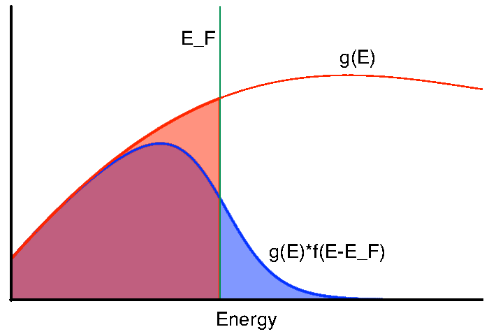
problem of system under finite temperatures. In fact one can show that
by simply approximating the step function with a Fermi-Dirac
distribution
-mesh convergence though one has to live with the
fact that the result obtained is actually for a slightly different
problem of system under finite temperatures. In fact one can show that
by simply approximating the step function with a Fermi-Dirac
distribution
![]() where
where
![]() we in general cannot get the integral
we in general cannot get the integral
![]() to equal to
to equal to
![]() exactly, this can be
seen clearly in figure 3
exactly, this can be
seen clearly in figure 3
 |
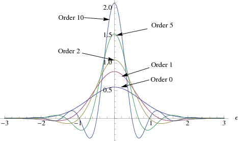
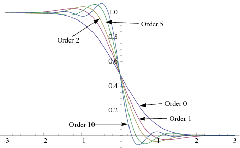
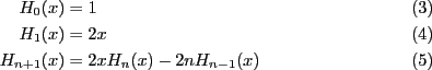
A more sophisticated approximation to the occupation function can be
done using Methfessel and Paxton method[14]. This
method approximates the step-function by starting with approximating
the delta-function using expansion in a set of orthogonal Hermite
polynomials. And then the ![]() -th order approximation
-th order approximation ![]() is
obtained by integrating the delta function. The method
guarantees that
is
obtained by integrating the delta function. The method
guarantees that
![]() for any
for any ![]() that is an polynomial of
that is an polynomial of ![]() -th order or less. The
expansion in Hermite polynomials are given as
-th order or less. The
expansion in Hermite polynomials are given as
where
| (4) |
The ground-state energy when calculated using Methfessel-Paxton
smearing is no-longer variational. Instead the ground-state density
minimises the free energy[11]
| (5) |
|
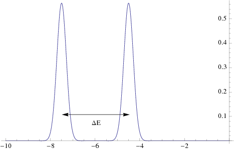
However Methfessel-Paxton method also introduces a numerical artefact
that Fermi-energy may no-longer be unique. To see this we notice that
by expanding the delta function in terms Hermite polynomials, we
introduce a number of roots to the function, and this translates into
regions of negative occupancies in ![]() . This is illustrated in
figure 4. As a result, the electron number as a
function of Fermi energy:
. This is illustrated in
figure 4. As a result, the electron number as a
function of Fermi energy:
| (6) |
 |
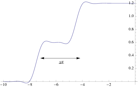 |
While given a lower bound and upper bound in function ![]() the bisection method always returns a solution
the bisection method always returns a solution ![]() that gives the
desired electron numbers, it is important that we are consistent on
which
that gives the
desired electron numbers, it is important that we are consistent on
which ![]() --if there are more than one--we actually find. Note that
the properties of non-unique Fermi energy is not physical, but is an
artefact of Methfessel-Paxton approximation. Never the less, to be
consistent in our calculations we define the Fermi energy to be
always the lowest energy that give the correct electron number.
--if there are more than one--we actually find. Note that
the properties of non-unique Fermi energy is not physical, but is an
artefact of Methfessel-Paxton approximation. Never the less, to be
consistent in our calculations we define the Fermi energy to be
always the lowest energy that give the correct electron number.
To make sure we always find the lowest energy solution, we need to
find the lower and upper energy bounds very carefully. To get a lower
bound, we could always start from the lowest energy. However to be
more efficient, this energy is probably too low, and we define a
parameter ![]() such that we fill up the lower bands (and assuming
occupation of 1.0) until we have
such that we fill up the lower bands (and assuming
occupation of 1.0) until we have ![]() electrons. And we use the
highest filled energy as the lower bound. To find the upper bound, we
increase the lower band by energy steps of
electrons. And we use the
highest filled energy as the lower bound. To find the upper bound, we
increase the lower band by energy steps of
![]() until
until
![]() is greater than the desired number of electrons. To find
is greater than the desired number of electrons. To find
![]() , we have to be careful the that it is not too big
and miss one possible solution and at the same time not too small so
that calculation is still efficient. We note that the width of the
Methfessel-Paxton approximation to delta function is controlled by the
gaussian weight
, we have to be careful the that it is not too big
and miss one possible solution and at the same time not too small so
that calculation is still efficient. We note that the width of the
Methfessel-Paxton approximation to delta function is controlled by the
gaussian weight ![]() , where
, where
![]() . Hence
we may define the width
. Hence
we may define the width ![]() of the Methfessel-Paxton approximation to
delta function as
of the Methfessel-Paxton approximation to
delta function as
| (7) |
![\begin{empheq}[box=\fbox ]{equation}
\delta \epsilon = \frac{W}{\eta2 N} = \frac{\sqrt{-\ln(g)}k_B T}{\eta N}
\end{empheq}](img104.png)