 |
Dr Ning Li
Numerical Algorithms Group (NAG)
Wilkinson House, Jordan Hill Road,
Oxford, OX2 8DR, UK
Date: March 18, 2010
There are two approaches to performing such computations on distributed-memory systems. One can either develop distributed algorithms (such as parallel tridiagonal solver or parallel FFT working on distributed data), or one can dynamically redistribute (transpose) data among processors in order to apply serial algorithms in local memory. The second approach is often preferred due to its simplicity: any existing serial algorithms (hopefully efficiently implemented already for a single CPU) remain unchanged; porting serial code can be quite straight-forward as much of the original code logic still holds, and the only major addition is the data transposition procedures.
|
In the past, many applications implemented the above idea using 1D domain decomposition (also known as `slab' decomposition). In Fig.1, a 3D domain is arbitrarily chosen to be decomposed in Y and X directions. It can be seen that in state (a), any computations in the X-Z planes can be done in local memories while data along a Y mesh-line is distributed. When it is necessary to calculate along Y mesh-lines (say to evaluate Y-derivatives, or to perform 1D FFTs along Y), one can redistribute the data to state (b), in which any computation in Y becomes `local'. Swapping between state (a) and (b) can be achieved using standard MPI_ALLTOALL(V) library.
A 1D decomposition, while quite simple, has some limitations, especially for large-scale simulations. Given a cubic mesh of size N3 , one obvious constraint is that the maximum number of processors Nproc that can be used in a 1D decomposition is N as each slab has to contain at least one plane. For a cubic mesh with 1 billion points, the constraint is Nproc < = 1000 . This is a serious limitation as most supercomputers today have more than 10,000 cores and some have more than 100,0001. Large applications are also likely to hit the memory limit when each processor handles too much workload.
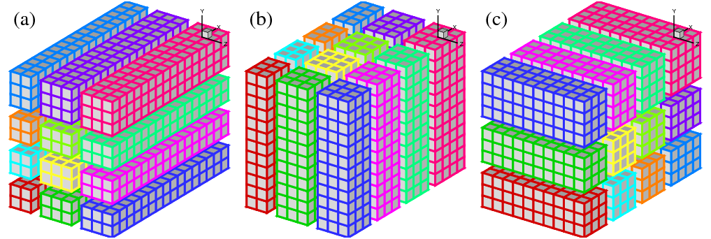
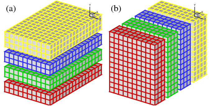
A 2D decomposition (also known as a `pencil' decomposition) is a natural extension to 1D decompositions. Fig.2 shows that the same 3D domain as in Fig.1 can be partitioned in two dimensions. From now on, states (a), (b) and (c) will be referred to as X-pencil, Y-pencil and Z-pencil arrangements, respectively. While a 1D decomposition algorithm swaps between two states, in a 2D decomposition one needs to traverse 3 different states using 4 global transpositions ( (a) - > (b) - > (c) - > (b) - > (a) ).
Again MPI_ALLTOALL(V) can be used to realise the transpositions. However it is significantly more complex than the 1D case. There are two separate communicator groups. For a Prow×Pcol processor grid: Prow groups of Pcol processors need to exchange data among themselves for (a) < - > (b) ; Pcol groups of Prow processors need to exchange data among themselves for (b) < - > (c) . It is also worth mentioning that the implementation of the communication routines are very sensitive to the orientations of pencils and their associated memory patterns. The packing and unpacking of memory buffers for the MPI library needs to be handled with great care (See Appendix A for details). These software engineering topics are almost certainly irrelevant to the scientific researches conducted by the software. This is one of the motivations to create the 2DECOMP&FFT library - to handle these technical issues properly and to hide all communication details from the application developers who can concentrate on their scientific studies.
The 2DECOMP&FFT library is delivered in a .tar.gz package. There is no special installation procedure - simply decompress the package in any directory and it is ready to be built. A Fortran 95 compatible compiler is the minimum requirement.2
A main Makefile template is provided to build the library, together with a few test applications. The library has been tested using several different compilers and compiler-specific flags are defined in the platforms subdirectory - one file for each compiler. Feel free to create new entries if testing this library on a new system - please send the author a copy as he is always interested in supporting the library on all major hardware platforms.
One may choose to turn on/off some software features in the main Makefile by appending flags to the OPTIONS variable. The available options are explained here:
For applications using the FFT interface, an FFT engine may be selected in the main Makefile . The multi-dimensional FFT routines delegate 1D transforms to a 3rd-party library. The default FFT engine (called 'generic') is based on an algorithm proposed by Glassman [2][5]. Also released in this version are implementations using FFTW3, ACML FFT and FFTPACK5.
A few test applications are provided which not only validate the communication code, but also serve as examples to demonstrate proper use of the library.
This section explains all the public interfaces of the 2D decomposition library. After reading this section, users should be able to easily build applications using this domain decomposition strategy. The library interface is designed to be very simple. One can refer to the test application (test2d.f90) for a quick start.
The library has been written in one Fortran module. So all applications should include this module at the beginning:
use decomp_2d
The public interface of the library includes a set of global variables containing the decomposition information - how the global data is distributed - which applications need to define their data structures. All these global variables should be read-only after being initialised by:
call decomp_2d_init(nx,ny,nz,P_row,P_col)
where nx
, ny
and nz
are the size of 3D global data to be distributed over a 2D processor grid
Prow×Pcol
. Note that none of the dimensions need to be divisible by Prow
or Pcol
. However, choose the numbers smartly to avoid significant load-imbalance, which could lead to poor performance. Also note that the constraints here are:
ProwFollowing is the list of global variables that can be used in applications. Obviously these names should not be redefined in applications to avoid conflict.4 Also note that some variables contain duplicate or redundant information just to simplify the programming.
It is recommended that an applications define its major data structures using these global variables in its main program immediately after initialising the decomposition library. Using allocatable arrays is preferred but it is also possible to use static arrays in subroutines, as shown in the following examples:
      ! allocate a X-pencil array
      allocate(var(xsize(1), xsize(2), xsize(3)))
      ! allocate a Y-pencil array using global indices
      allocate(uy(ystart(1):yend(1), ystart(2):yend(2), &
                  ystart(3):yend(3)))
      ! define a Z-pencil work array in a subroutine
      real, dimension(zsize(1),zsize(2),zsize(3)) :: work1
The library also contains a set of communication routines that actually perform the data transpositions. As mentioned in Section 2, one needs to perform 4 global transpositions to go through all 3 pencil orientations. Correspondingly, the library provides 4 communication subroutines:
      call transpose_x_to_y(in, out)
      call transpose_y_to_z(in, out)
      call transpose_z_to_y(in, out)
      call transpose_y_to_x(in, out)
The input array in and output out should have been defined for the correct pencils in the calling program. Note that the library is written using Fortran's generic interface so different data types are supported without user intervention. For many applications both arrays simply contains real numbers. But in and out can be complex arrays for FFT-type of applications.
Although it is not necessary for application developers to understand the internal logic of these transposition routines, it is important to know that they can be expensive, especially when running on large number of processors. So applications should minimize the number of calls to them, even sometimes at the cost of duplicating computations.
Finally, before exit, applications should clean up the memory by:
call decomp_2d_finalize
FFTW[1] is one of the most popular FFT packages available. It is open-source, supporting arbitrary input size, portable and delivers good performance due to its self-tuning design (planning before execution). There are two major versions of FFTW. Version 2.x actually has a reliable MPI interface to transform distributed data. However, it internally uses a 1D (slab) decomposition which, as discussed earlier, limits the scalability of large applications. Its serial performance is also inferior to that of version 3.x, which has a brand-new redesign that has better support to SIMD instructions on modern CPUs. Unfortunately, the MPI interface of version 3.x is in unstable alpha stage and has been so for many years. So there is no reliable way to compute multi-dimensional FFTs in parallel.
CRAFFT (CRay Adpative FFT) is available on Cray systems, for example, as part of xt-libsci library on XT systems. It provides a simplified interface to delegate computations to other FFT kernels (including FFTW). Being `adaptive' means that it can dynamically select the fastest FFT kernels available on a system. However, it only supports very limited distributed routines (only 2D/3D complex-to-complex transformations are supported as of version xt-libsci/10.4.0) and those routines are based on an evenly-distributed 1D decomposition.
It is well known that a multiple-dimensional FFT is equivalent to a series of 1D FFTs. Having developed the communication library, one obvious approach to perform multiple-dimensional FFTs on distributed machines is to use established libraries like FFTW (or whatever libraries are tuned specially for your hardware) to efficiently compute 1D FFTs in local memory and rely on the communication library to perform global data transpositions. An FFT interface has been developed on top of the communication library to implement this idea.
First of all, one additional Fortran module has to be referred to in order to use the FFT interface.
use decomp_2d_fft
As mentioned earlier, the FFT interface is built on top of the decomposition library, which, naturally, needs to be initialised first.
call decomp_2d_init(nx,ny,nz,P_row,P_col)
Then one needs to initialise the FFT interface by:
call decomp_2d_fft_init
By default, it is assumed that physical-space data is stored in X-pencil. The spectral-space data is then stored in transposed Z-pencil format after FFT. To give applications more flexibility, the library also supports the opposite direction, if an optional parameter is passed to the initialisation routine:
call decomp_2d_fft_init(PHYSICAL_IN_Z)
Physical-space data in Y-pencil is not an option as it would require additional expensive transpositions which does not make economical sense.
The main function this FFT package provides is to perform 3D FFTs where the distributed input data is stored in ordinary ijk-ordered 3D arrays across processors. For complex-to-complex (c2c) FFTs, the user interface is:
call decomp_2d_fft_3d(in, out, direction)
where direction can be either DECOMP_2D_FFT_FORWARD for forward transforms, or DECOMP_2D_FFT_BACKWARD for inverse transforms. The input array in and output array out are both complex and have to be either a X-pencil/Z-pencil combination or vice versa, depending on the direction of FFT and how the FFT interface is initialised (PHYSICAL_IN_X, the optional default, or PHYSICAL_IN_Z).
While the c2c inteface is already in the simplest possible form, for many applications using real numbers only, the 3D FFT interface can be used in a more compact form:
call decomp_2d_fft_3d(in, out)
Here if in is a real array and out a complex array, then a forward FFT is implied. Similarly a backward FFT is computed if in is a complex array and out a real array.
When real input is involved, the corresponding complex output satisfies so-called `Hermitian redundancy' - i.e. some output values are complex conjugates of others. Taking advantage of this, FFT algorithms can normally compute r2c and c2r transforms twice as fast as c2c transforms while only using about half of the memory. Unfortunately, the price to pay is that application's data structures have to become slightly more complex. For a 3D real input data set of size nx×ny×nz , the complex output can be held in an array of size (nx/2 + 1)×ny×nz , with the first dimension being cut roughly in half (for PHYSICAL_IN_Z, the complex output is of size nx×ny×(nz/2+1) instead)5. For parallel computing, these arrays of smaller sizes have to be distributed as 2D pencils and such distribution is different from the distribution of nx×ny×nz arrays - additional internal data structures are required in the library to handle this. 2DECOMP&FFT library hides as many such details as possible from users and only provides one utility subroutine to help applications properly allocate memory space when using the r2c/c2r interface. The syntax is:
call decomp_2d_fft_get_dims(start,end,size)
where all three arguments are 1D array of three elements, returning to the caller the starting index, ending index and size of the sub-domain held by the current processor - information very similar to the start/end/size variables defined in the main decomposition library discussed in Section 4 but covering a different global domain. The returning values are also dependent on how the FFT interface is initialised. By default they describe the storage of the distributed complex output in Z-pencil. However, if PHYSICAL_IN_Z is used at initialisation, X-pencil representation is returned. Please note that the complex output arrays obtained from X-pencil and Z-pencil input do not contain identical information. However, if `Hermitian redundancy' is taken into account, no physical information is lost and the real input can be fully recovered through the corresponding inverse FFT from either complex array.
Finally, to release the memory used by the FFT interface:
call decomp_2d_fft_finalize
It is possible to re-initialise the FFT interface in the same application at the later stage after it has been finalised, if this becomes necessary. To obtain first-hand experience on the FFT interface, users are advised to examine the two sample applications (fft_test.f90 and fft_test_r2c.f90) distributed with the library.
As shown in the earlier sections, the underlying communication library is both flexible and powerful and it is possible to build on top of it additional functionalities.
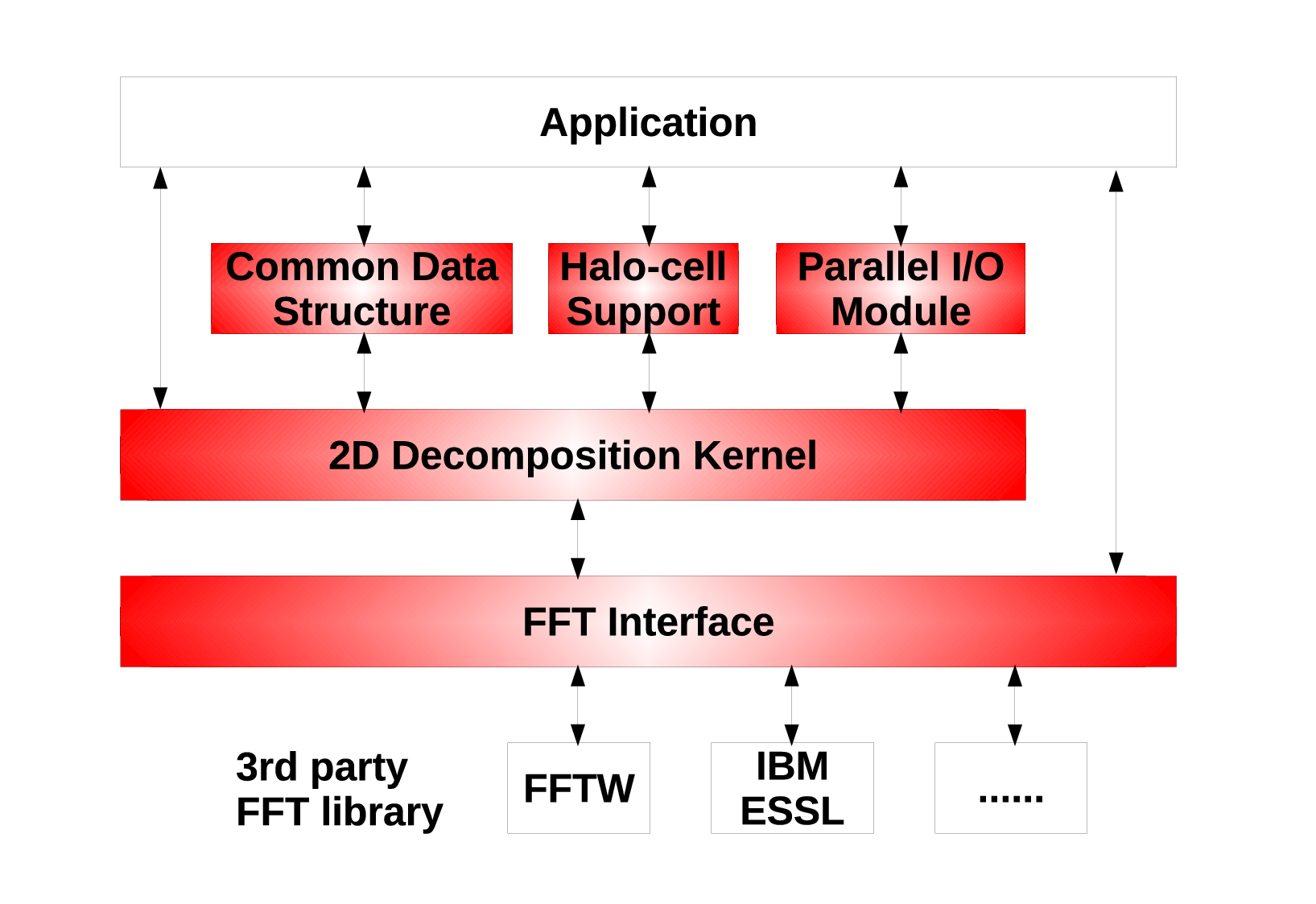
Fig. 3 shows a blueprint of an extended library, with includes functional modules already available in 2DECOMP&FFT, as well as additional supporting modules which might be useful for applications.
The kernel of the library provides the basic domain decomposition information and data transposition routines - the minimum an application will need to use the 2D decomposition strategy.
The FFT interface provides user-friendly access to multiple dimensional FFTs. It handles the data management and delegates 1D FFTs to whatever optimised FFT libraries available on each hardware.
Some additional functional modules can be provided between the communication kernel and the applications to further simplify the building of applications. A few useful modules are shown in the blueprint:
The performance of a distributed FFT library is determined by both the computation efficiency of the underlying 1D FFT algorithm and the communication efficiency of the data transposition algorithm. The following table shows the speed-up this library can achieve over the serial runs using FFTW's 3D FFT interface. The times reported (in seconds) are for forward c2c transforms and all the transforms were planned using FFTW_ESTIMATE.
| Data size N3 | Serial FFTW | Parallel 2DECOMP&FFT | |||
| Planning | Execution | 16 cores | 64 cores | 256 cores | |
| 643 | 0.359 | 0.00509 | 0.00222 | - | - |
| 1283 | 1.98 | 0.0525 | 0.0223 | 0.00576 | 0.00397 |
| 2563 | 8.03 | 0.551 | 0.179 | 0.0505 | 0.0138 |
| 5123 | 37.5 | 5.38 | 1.74 | 0.536 | 0.249 |
| 10243 | - | - | - | 4.59 | 1.27 |
| 20483 | - | - | - | - | 17.9 |
It can be seen that due to the communication cost, the absolute speed-up over the serial library isn't great (only about 20-40 times on 256 cores). However, the parallel library does allow much larger problems to be computed quite efficiently. In particular, for smaller core count (16 and 64), each time the problem size is increased by 8 times, the computing time increases by 8-10 times, following the trend of the underlying serial library very well.
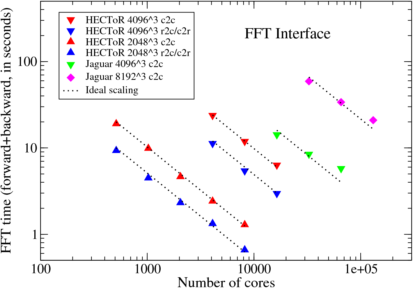
Some large-scale parallel scaling benchmarks of the FFT interface were done on HECToR and Jaguar6, using problem size up to 81923 . The timing results presented here are the time spent to compute a pair of forward and backward transforms on a random signal, both c2c and r2c/c2r. The underlying FFT engine is the latest version of ACML FFT. In all cases, the original signals were recovered to machine accuracy after the backward transforms - a good validation for the library itself. Up to 16384 cores were used on HECToR and each case was repeated 3 times and the fastest results were recorded. On Jaguar, the world No. 1 system at the moment, fewer but larger tests were arranged using up to 131072 cores. Please note that runtime does vary a lot for communication intensive jobs on busy systems.
It can be seen that the FFT interface scales almost perfectly on HECToR for all the tests done. On Jaguar, the scaling is less good for larger core counts but the efficiency is still at a respectable 81% for the largest test. It took Jaguar more than twice of time to run the only common test on both systems, a 16384-core job on the 40963 mesh. This is not unexpected. While HECToR has quad-core processors at the moment, Jaguar has two 6-core chips built on each node. The problems set up for these benchmarks really prefer a power-of-2 core count to run efficiently as the communication network can be used in a more balanced way. More in-depth performance studies will be conducted (hopefully on several other supercomputing facilities) when the major development works of 2DECOMP&FFT are completed.
This library development is supported through a distributed CSE support project on HECToR. The collaborating academic partner is the Imperial College based Turbulence, Mixing and Flow Control group. The project is to modernise the group's CFD application Incompact3D which is a finite difference code using high-order compact schemes for Direct and Large-eddy Simulations (DNS/LES)[6]. The original Incompact3D was based on 1D decomposition which became a bottleneck once the group started doing large-scale simulations using at least a few billion mesh points. The new Incompact3D has been built on top of the 2D decomposition library and some preliminary performance result is shown in Fig. 5
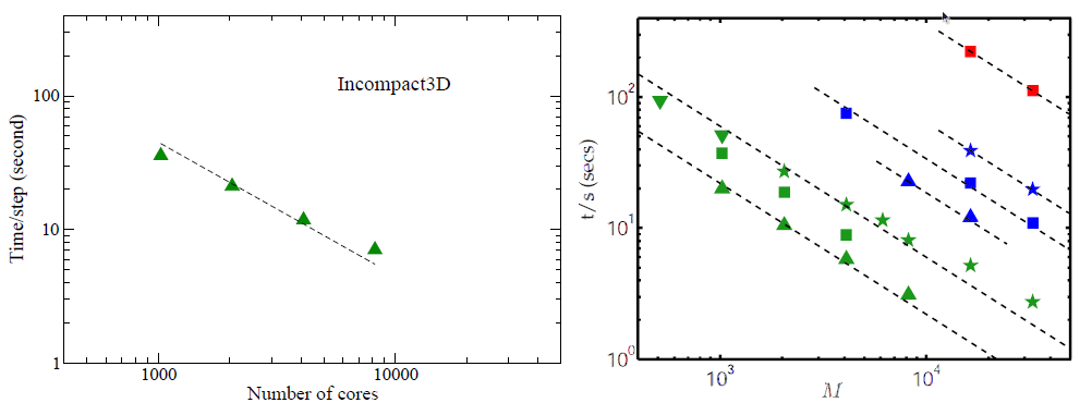 |
A DNS was set up on a mesh of 20483 points and ran on HECToR using up to 8192 cores. The scaling efficiency archived is 89.4% between 2048 and 4096 cores and 83.6% between 4096 and 8192 cores. In comparison, the scaling results of P. K. Yeung's spectral DNS code[4] based on P3DFFT library are reproduced here. What is directly comparable is the data set taken from supercomputer Franklin (also a Cray XT4) shown as green triangles, exhibiting very similar scaling behaviour. More details are given in the following table.
| Number of cores | Time/step(sec) | 2D processor grid | % user code |
| 1024 | 35.7 | 2×512 | 54% |
| 2048 | 21.1 | 2×1024 | - |
| 4096 | 11.8 | 4×1024 | - |
| 8192 | 7.06 | 8×1024 | 38% |
The percentage of user code was recorded using CrayPAT, the Cray Performance Analysis Tool. As expected, the application becomes more communication intensive as the number of cores increases. It is also seen that the communication library performance is highly dependent on the proper selection of the 2D processor grid, which will be discussed later in Section 7.3.
In addition to the finite difference part of the code, which relies on global transpositions to solve tridiagonal systems derived from discretising the Navier-Stokes equations, Incompact3D also includes an algorithm to solve the pressure Poisson equation in spectral space. This is an innovative idea in which a Fourier-based spectral method can be applied to a wider range of applications without the constraint of periodic boundary conditions. The algorithm is based on pre- and post-processing of data in both physical and spectral spaces before and after normal 3D FFTs. As a result, it can directly take advantage of the works done in the parallel FFT library. The pre- and post-processing procedures themselves sometimes contain global operations which require data transposition routines in the base library. Currently, work is being carried out to build the Poisson solver on top of the FFT library. Additional benchmarks are being planned and carried out on HECToR and other supercomputers and further results will be available at a later time.
The global transpositions and MPI_ALLTOALL type of communications are known to be very demanding for network bandwidth. So it is almost certain that large applications can run faster on multi-core chips if not using all the cores from each physical node. This may also improve the computational efficiency due to improved memory bandwidth. Unfortunately this is rarely practical on most supercomputers where the resource charging is on per-node basis. Shared-memory programming, as will be discussed in Section 8, may improve the situation.
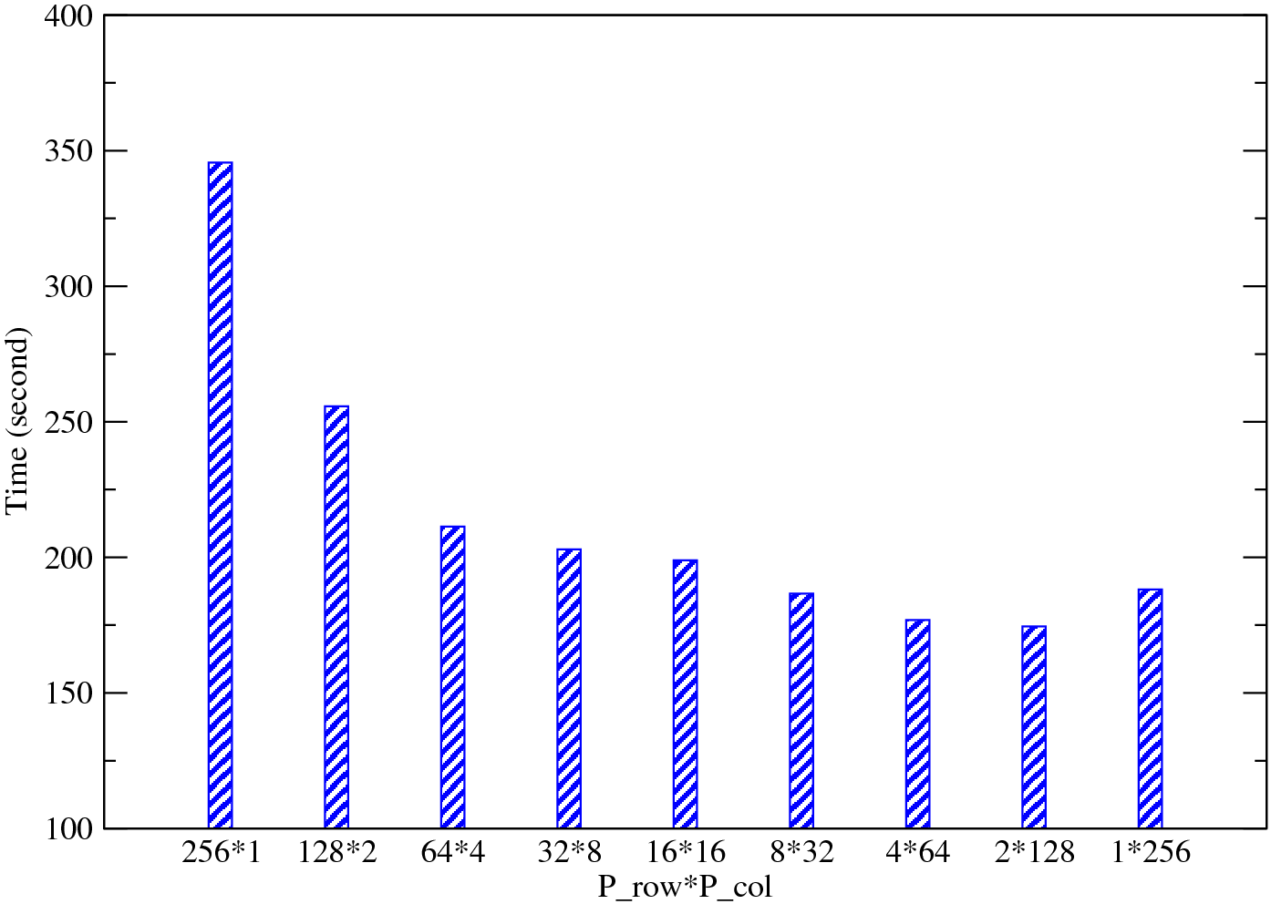
Application users need to be aware that they have the freedom to choose the 2D processor grid Prow×Pcol when using this library. Depending on the hardware, in particular the network layout, some processor grid option deliver much better performance than others. Application users are highly recommended to test this issue before running large simulations. An auto-tuning algorithm may be included in future releases to allow the best processor grid to be determined at runtime.
Fig. 6 shows the performance of a test application using 256 MPI ranks on HECToR. It can be seen that subject to constraint max(Prow, Pcol) < min(nx, ny, nz) , Prow < < Pcol is the best possible combination for this particular hardware (using Torus interconnection network). There are several technical reasons for such behaviour. First of all the hardware was equipped with quad-core processors (4-way SMP). When Prow is smaller than or equal to 4, half of the MPI_ALLTOALLV communications are done entirely within physical nodes which can be very fast. Second, as the communication library only handles ijk-ordered arrays, larger nx/Prow tends to use the system cache more efficiently. The 1*256 case is effectively a 1D decomposition, although still using the 2D data structure and code logic. Theoretically, it can be even faster if simplified data structure and code logic are used. This may be implemented in a future release.
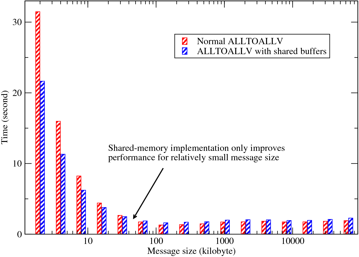
For the ALLTOALL type of communication in which each MPI rank has to send/receive messages to/from all other MPI ranks, one can imagine that traffic from cores on the same physical node compete for their network interface. One possible solution is to create shared send/recv buffers on each SMP node. Then only leaders of the nodes participate MPI_ALLTOALL(V), resulting in fewer but larger messages passing within the system, hopefully improving the performance of communication.
The actual shared-memory program was based on code supplied by David Tanqueray of Cray Inc. who initially applied this idea to several molecular dynamics applications. The shared-memory code uses the Unix System 5 shared memory API which is widely supported (try man shmget at command line to see if it is available on your system). Similar to the standard library, the shared-memory library has been implemented as a black box. So user can simply use `-DSHM' flag when compiling the library to switch it on.
Please note that this shared-memory implementation isn't automatically portable while moving to a new system. Cray XT is currently the only supported system. There is a piece of low-level code (function get_smp_map_ in alloc_shm.c) which accesses system-dependent information to gather vital information for the share-memory code (such as which MPI rank belongs to which node)8. This function needs to be rewritten for different hardware. However, one can reasonably expect that such function can be provided by hardware suppliers or system administrators familiar with the new hardware. Please contact the developer if you can help port this code to a new system.
Finally, the performance of the shared-memory code is shown in Fig. 7. The data was collected on HECToR from a series of simulations using 256 MPI ranks over a range of problem sizes. When the problem size is small (so is the message size), the transposition routines were called more times so that the total amount of data moving within the system remains a constant. Fig. 7 shows that when the problem size is small, the overhead of setting up communications is very high and the shared-memory code can improve communication efficiency by up to 30%. As the problem size increases, the benefit of using shared-memory code becomes smaller. In fact for large message size (> 32Kb in this example), the shared-memory code is actually slower due to the extra memory copying operations required (see Appendix A for details if you are interested). However, do remember this test was performed on a quad-core system. HECToR is scheduled to be upgraded to 24-core system in 2010 and the general trend across major supercomputing sites is to have more cores per node. Do expect the shared-memory code to play a more significant role in the near future.
The developer is particularly interested in working on real-world applications that may benefit from this work. Please feel free to contact him to discuss collaboration opportunities.
These are a collection of more in-depth technical topics which are mainly for advanced users and developers.
The communication library always handle ijk-ordered input and output. The memory pattern of such arrays are often different from the memory pattern required by the MPI_ALLTOALL(V) buffers. This section documents details on how proper packing and unpacking of these buffers can be implemented in the communication routines.
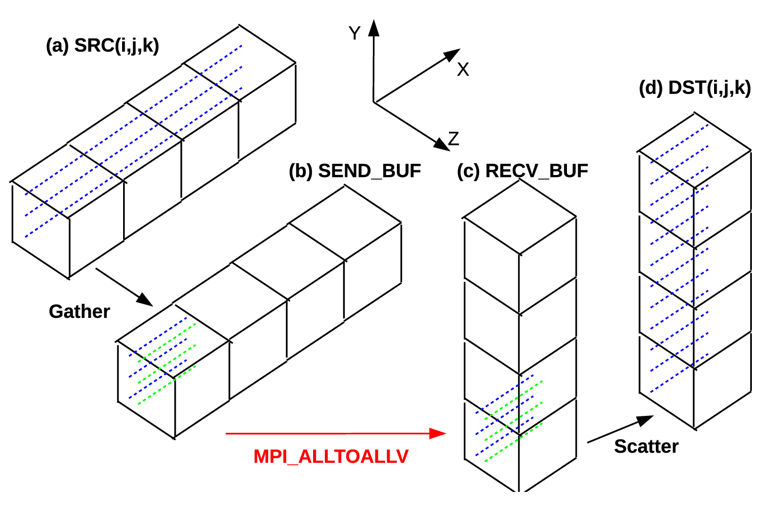
Fig. 8 illustrates the transposition between X- and Y-pencils. As can be seen, the send buffer in Fig. 8(b) consists of 4 subsections each containing data to be sent to different MPI ranks and data for each subsection has to be gathered together in memory (although the internal storage order does not matter). Obviously the memory pattern of the input data, shown in Fig. 8(a), does not satisfy such requirement as data along the dotted lines are contiguous in memory in a normal Fortran multi-dimensional array. The packing (or gathering) of the send buffer can be achieved in several ways. For example, an index-rotating procedure can be applied to the input, changing it to a jki-order array, which is suitable to be a send buffer. In practice, such index rotating proved to be very inefficient. A far better approach is to keep the data in each subsection in normal ijk-order by copying data segment by segment from the input array. This will copy roughly nx/Prow number of contiguous data point at a time, which is much more cache-friendly. At the receiving end, a similar unpacking (or scattering) operation needs to be applied.
Transpositions between Y- and Z-pencils are similar. But one special feature is that the receive buffer shown in Fig. 9(c) is automatically in an ijk-order so that the scattering operation becomes unnecessary, resulting in fast communication routines. This also explains why the shared-memory code takes longer time to run in Fig. 7 - packing and unpacking the shared buffer is always necessary and savings achieved here do not apply in that situation.
Based on the discussions here, further performance-improvement measures may be taken in certain applications. As can be seen, memory copying between Fig. 8(c) and (d) is exactly the opposite of that between Fig. 9(a) and (b). If it is possible in applications to carry out whatever Y-pencil operations using the buffer data structure rather than the normal ijk-ordered data structure, then both sides of memory copying operations can be saved. More general communication routines may be implemented if there is such requirement.
To complete 3D FFT computations, multiple 1D FFTs need to be performed in each dimension. It is possible to rely on simple 1D FFT algorithm only - the idea is for applications to loop through all 1D data sets stored in 3D data structures, copy them into 1D buffers of proper format, before calling 1D FFT routines. For efficiency reason, well-known 3rd-party FFT libraries often provide more complex user interfaces that enable multiple 1D FFTs to be computed in one go. This is the case in FFTW's advanced interface and ACML FFT's expert driver.
Using such advanced user interface, one needs to specify two major parameters to describe the memory pattern of the input/output data structures: (1) A stride variable that describes how far each point in a 1D data set is separated in memory; (2) A distance variable that describes how far each 1D data set is separated in memory.
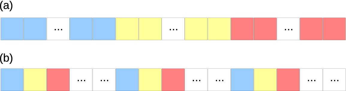 |
Fig. 10(a) shows the memory pattern of 1D data sets aligning in X direction. For natural ijk-ordered arrays, as the first index changes fastest in Fortran, data sets in X has a stride of 1 with each separated by nx , the size of the 3D array in X. Fig. 10(b) shows the memory pattern of 1D data sets aligning in Z direction. As the 3rd dimension changes the slowest, neighbouring data points in Z are separated by nx×ny (the stride) and each set is shifted only by 1 point. The data sets in Y have a similar pattern as in Fig. 10(b) but only on each Z-plane. So 1D FFTs in Y need to be done within a loop over Z planes.
This document was generated using the LaTeX2HTML translator Version 2008 (1.71)
Copyright © 1993, 1994, 1995, 1996,
Nikos Drakos,
Computer Based Learning Unit, University of Leeds.
Copyright © 1997, 1998, 1999,
Ross Moore,
Mathematics Department, Macquarie University, Sydney.
The command line arguments were:
latex2html -split 0 -no-navigation -show_section_numbers -html_version 3.2,math -no-math -antialias UserGuide
The translation was initiated by Ning Li on 2010-03-18