2D domain decomposition

Fig 1 shows the schematic difference between a one dimensional decomposition and a two dimensional decomposition of the global grid. The 2D decomposition increases the number of MPI tasks with a factor equal to the number of rows used, but because the spatial derivatives are computed with an implicit rule, one more transpose operation along the x axis is needed in the case of a 2D decomposition. Nevertheless for large grids and a high speed communications network, this procedure is scalable.

The implementation of the 2D domain decomposition is straightforward with the help of the 2DECOMP library [2]. The calls to subroutines used for the $y\leftrightarrow z$ transposed provided in the original code were replaced with calls to the corresponding transpose_y_z subroutines of the 2DECOMP library. In the case of the x derivative, which needs a $y \leftrightarrow x$ transpose the subroutine that computes the derivative was extended to perform the transpose operation if needed ( this is determined from the analysis of the local grid dimensions). The possibility to use a 1D decomposition is preserved, in this case the code skips any $y \leftrightarrow x$ transpose operation thus preserving the performance of the initial version.

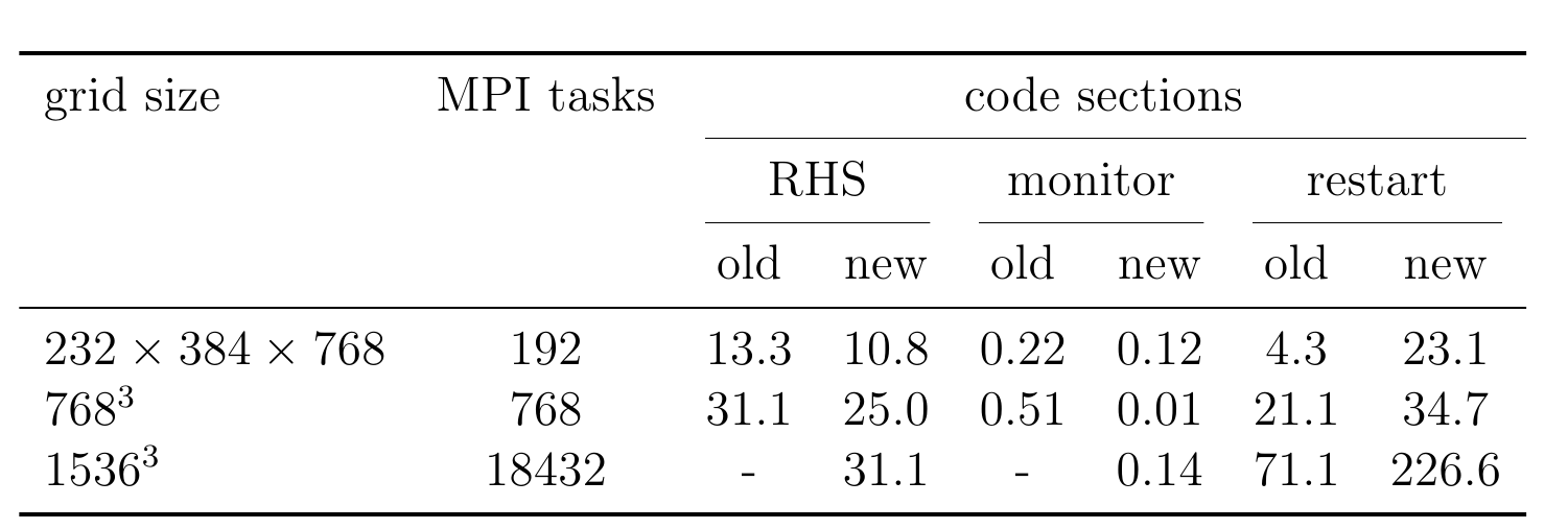
The scalability of the 2D decomposition algorithm was tested on two cubic grids with linear sizes 768 and 1536 using up to 18432 MPI tasks. The number of processor rows used in the processor grid was set to 24 or 48 in order to keep the data movement for the $y \leftrightarrow x$ transpose inside a node or only between two nodes.

Figure 2 shows the computation time per grid point (normalised to the size of a 768 cubed grid) of the core solver subroutine (RHS) which in for a typical production run will consume more than 90% of the computation time. The plot shows that the 2D decomposition has a good scaling up to 18432 MPI tasks with approximately a 50% efficiency for the grid size 1536 using 48 rows for the MPI task grid. An interesting crossover phenomenon is worth mentioning here. The performance of the 2D decomposition with 24 processor rows is better at small core counts: (3072 MPI tasks for the 768 cubed grid and 4608 MPI tasks for the 1536 cubed grid) but the decomposition that uses 48 processor rows has better performance at larger numbers of MPI tasks for both grid sizes (other tested values for the number of rows show significantly lower performance).

It has not escaped our notice that on a parallel computer with largely multicore nodes, an alternative algorithm can be used to increase scalability: one can keep the original 1D decomposition of the simulation grid, thus saving a significant amount of communication, and increase the speed of computation with the help of OpenMP threads in each local grid.

A prototype implementation of this algorithm was implemented, together with a thorough study of scalability. This work was presented at the Cray user Group conference 2011 [3]. The main conclusion of this study is that a mixed mode 1D decomposition is at least 20% faster than a 2D decomposition at a cost of more complicated code, see Fig 2, even better results area achievable if overlapping between communication and computation is done with the help of OpenMP threads¹.

Table 1: Timings for the pre-dCSE version and the current one for three grid sizes. Data are for the right hand side term computation (RHS) (seconds per step), monitoring (seconds per operation) and one restart (read and write). The first two models use a 1D decomposition, the last one uses a 2D decomposition with 48 processor rows. The pre-dCSE code cannot run the largest grid because of insufficient memory, the restart time was obtained on the current version with the Fortran IO switched on. The restart files for the MPI-IO version use 1, 32 and 64 stripes, respectively.

---------------------------------------------------------------------------------
---------------------------------------------------------------------------------