Background and pre-dCSE code overview

For the last 20 years, DSTAR has been used, in original and modified versions, by a number of researchers who have worked closely with Prof. Kai Luo on turbulence and combustion simulations with the direct numerical simulation method. These include: Prof. Neil Sandham and Dr. Zhiwei Hu (University of Southampton), Prof. Xi Jiang (University of Lancaster), Dr. Eldad Avital (Queen Mary, University of London), Dr. Yongman Chung (University of Warwick) and Dr. Jun Xia (Brunel University).

The system of partial differential equations that sets the mathematical frame for DSTAR and the numerical algorithms for their solution are described in detail in Ref [1]. In short, implicit compact finite difference schemes are employed for spatial discretisation with sixth-, fourth- and third-order schemes for internal, near-boundary and boundary points, respectively. A fourth-order Lagrangian interpolation scheme is utilised to obtain gas properties at droplet locations. A third-order explicit Runge-Kutta scheme is used for temporal advancement of the flow variables, while a semi-analytical scheme is employed for droplet marching, with the consideration of numerical accuracy, stability and efficiency.

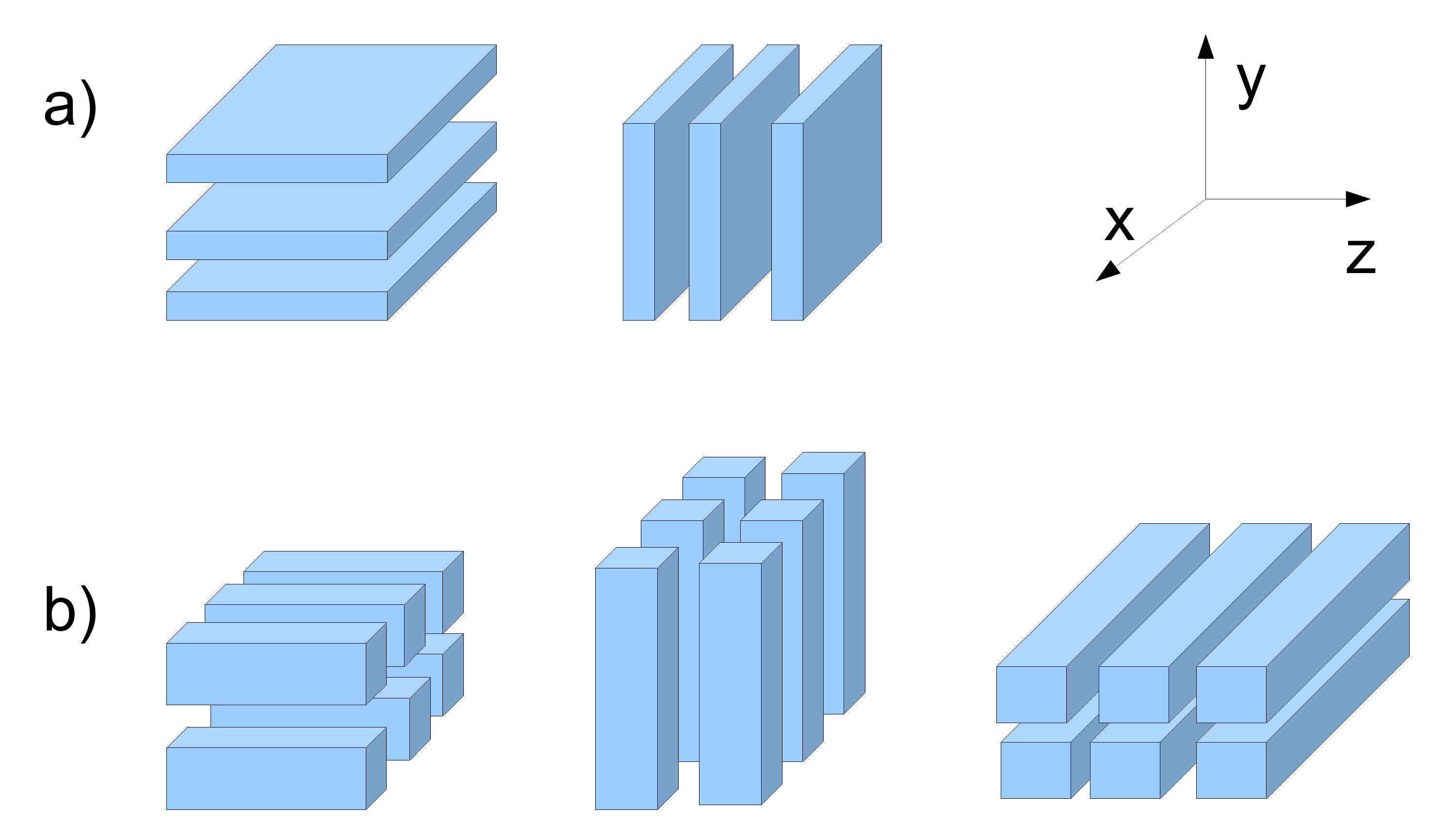
In the pre-dCSE version of DSTAR the parallel computation utilised a primary Cartesian grid, which was partitioned uniformly over the MPI ranks along the y axis (1D decomposition). Because the spatial derivatives are computed with an implicit rule, each MPI rank also needs a local grid which spans the whole domain along the y axis, hence a secondary partition along the z axis is also needed. Data between the two partitions are exchanged by transpose operations among all the MPI ranks, see Figure1 a).

The numerically intensive work which is done in DSTAR takes more than 90% of the run time for a typical run. This is concentrated within the subroutine which computes the right hand side terms (RHS) for the set of differential equations in time. These equations describe the evolution of the flow variables after spatial discretisation of the continuum field equations. The RHS set of subroutines contains mainly loops that perform updates to the flow variables, together with some derived quantities inside the domain and at the boundaries. Additionally, calls to subroutines that compute the spatial derivatives and calls to communication subroutines for the transpose operations described earlier are also included.

This section of the code has a large degree of parallelism due to locality of the update rule and the multicomponent nature of the discretised flow variables. On the other hand, for a global grid with dimensions N_x, N_z, N_y the number of processors that can be used in a 1D domain partition is limited by $min(N_y,N_z)$, which could be significantly smaller than the number of processing elements available on today's top supercomputers.

The input, output operations for the monitoring and the checkpoint data files were done with Fortran IO in multiple files, the monitoring data was collected in (ASCII) text files, one per observation point, the restart data was collected in binary files associated with subgroups of MPI tasks.

The source code files included a significant proportion of Fortran 77 files, many of them using implicit data declarations. The grid dimension and the number of MPI ranks were hard wired in an include file, thus making it necessary to recompile the source code if any of these parameters was changed.

Figure 1: Schematic representation of the domain decompositions required by DSTAR: a) 1D case with 3 MPI ranks along the z and y directions, b) 2D case with $3\times 2$ MPI ranks along the z, y and x directions; in this case a transpose along the x axis is also needed. Data exchange between decompositions require all to all type of communication.

Figure 2: Performance of the core solver subroutine (RHS) versus total number of MPI ranks in the case 2D decomposition with 24 and 48 processor rows for two cubic grids with linear size 768 and 1536. Note the crossover for both grids as the total number of ranks increases. Also shown is the performance of the mixed mode code (MM) which uses a fixed 1D decomposition with 768 and 1536 MPI tasks for each grid, respectively, but with increasing number of OpenMP treads.