


Next: 4. Refinement
Up: Multigrid Improvements to CITCOM
Previous: 2. Initial Project Study
Contents
Subsections
3. Multigrids
In order to solve a system of linear equations, typically one of the following two classes of
solvers is used.
- Direct methods
- Iterative methods
Direct methods originate from Gaussian elimination, they have a limited application field and
determine the solution at machine precision accuracy with optimal performance of
 [7] where n is the number of equations/unknowns in the
linear system.
[7] where n is the number of equations/unknowns in the
linear system.
Iterative methods have wider field of applications with Jacobi, Gauss-Seidel and Conjugate Gradient
being the most popular amongst others. However, attempts to overcome the unconvincing time
efficiency of these methods resulted in an extension to iterative methods called multigrid methods.
3.1 Multigrid Methods
Multigrid (MG) methods are a branch of numerical analysis and comprise of algorithms for systems of
linear equations typically obtained after the discretization of partial differential
equations. Elliptic partial differential equations are the prime candidates for the multigrid
algorithms/applications. These algorithms employ a hierarchy of discretizations at more than one
level of underlying grid. The purpose of these algorithms is that at multiple grid levels, called
multigrids, they accelerate the rate of convergence. This acceleration is achieved by employing a
number of steps in a specific order and includes:
- Relaxation/Correction of the global solution by solving a coarse grid problem
Helps
reduce high frequency errors by employing Gauss-Seidel like iterative methods, beginning at the
finest grid and gradually moving down to the coarsest grid where it becomes a coarse grid
problem.
- Restriction/Projection of the residual vector of the current approximation from a fine grid to
a coarse grid
Restricts/Projects down the residual vector to a coarse grid by employing
some form of averaging, for example.
- Prolongation/Interpolation of the approximation to a residual vector from a coarse grid to a
fine grid
Prolongates/Interpolates an approximation to the residual (error) at the coarse
grid to a fine grid and is used for correction there.
These three steps are building blocks or components of any multigrid algorithm and each of these
component is briefly described below.
3.1.1 Relaxation/Correction
It has been established [4] that many standard iterative methods possess the smoothing
property. This property makes these methods very effective at eliminating the high frequency or
oscillatory components of the error and leaves the low frequency or smooth (less oscillatory)
components relatively unchanged. These iterative methods can be further improved to handle error
components of all types equally effectively. Towards this end, relaxation schemes can be improved by
using a good initial guess. A well known technique to obtain a good initial guess is to perform a
few preliminary iterations on a coarse grid. As there are fewer unknowns on a coarse grid,
relaxation is less expensive and the rate of convergence on a coarse grid is marginally better as
well [4]. Further, a coarse grid solver also takes advantage of the fact that smooth
or low frequency components of error on a fine grid take the form of oscillatory or high frequency
components of error on a relatively coarse grid. In other words, when a relaxation scheme on a fine
grid begins to stall due to smooth error modes, it is the time to move to the coarse grid where
these error modes appear more oscillatory and the relaxation scheme becomes more effective. A
combined effect of this, along with other MG components, results in a substantial improvement to the
rate of convergence of the global problem.
In this context, consider the following steps:
- Relax on fine grid for an approximation to solution.
- Compute residual vector of the current approximation at fine grid.
- Transfer this computed residual vector to the coarse grid by means of a restriction operator.
- Relax on residual equation on coarse grid to get an approximation to error.
- Transfer this error approximation to fine grid by interpolation operator.
- Correct the approximate solution obtained on fine grid with error approximation at coarse
grid.
This procedure outlines the correction scheme. Theoretically, relaxation is employed on a fine grid
to approximate the solution until convergence stagnates or deteriorates. In practice, relaxation is
applied only for a few steps instead of waiting for convergence to stagnate or deteriorate. This
helps optimise MG schemes. However, the optimal choice of the number of steps that relaxation is
applied may vary for different problems. Relaxation is then applied to the residual equation on the
coarse grid to get the approximation to the error itself which is then used to correct the solution
approximation already obtained on fine grid. This fine grid and coarse grid scenario when extended
to more than at least two grid levels refers to multigrid and requires transferring the residual
vector to multiple levels in the grid hierarchy, from the finest grid to the coarsest grid via
intermediate grids. The same procedure is required to transfer approximations to the residual
(error) but in a reverse order, from coarsest grid to finest grid. These inter-grid transfer
procedures are referred as restriction/projection and prolongation/interpolation respectively.
As improvements to prolongation and restriction operators (along with the mesh refinement) are
topics of study planned for phase 3 (the next phase) within this project, these are not discussed
here except the description of the basic functionality of each of these operators for the sake of
completeness.
3.1.2 Prolongation/Interpolation
Prolongation/Interpolation, in the multigrid context, is an operator used to transfer error
approximation from coarse grid to fine grid. It can be of any order but even the simplest, linear
interpolation for example, works quite effectively.
3.1.3 Restriction/Projection
As the interpolation operator is used to transfer the error approximation from a coarse grid to a
fine grid, an operator with the reverse or counter effect that transfers the residual vector from
fine grid to coarse grid is called a restriction/projection operator. The most obvious example for
such an operator is the so called injection whereas a more elaborate alternative operator is the
full weighting or weighted average.
3.2 Multigrid Cycles
Multigrid schemes available within CITCOM at the end of this phase (phase 2) are described in this
section. The first two schemes implemented in CITCOM are known as multigrid V-cycle and W-cycle
schemes. The next two schemes are known as Full Multigrid or FMG schemes, these can also be referred
to as F-cycle schemes. Based on V-cycle and W-cycle within the FMG scheme, these are referred as
FMG(V) and FMG(W) schemes respectively.
3.2.1 V-cycle
Starting at the finest grid, the V-cycle scheme involves a number of relaxation steps followed by
computation of a residual vector which is than transferred to the next coarser grid with the help of
a restriction operator. This procedure is repeated until the coarsest grid with a relatively few
grid points (in comparison to the finest grid) is reached. This scheme then works its way back to
the finest grid while employing the correction just computed to the next fine grid which is
transferred by means of the prolongation operator. This procedure is repeated until the finest grid
is reached. At this point one iteration of the V-cycle is completed. A graphic representation of a
V-cycle iteration is shown in figure 3.1.
Figure 3.1:
Multigrid V-cycle Scheme
|
|
After each completed iteration of the V-cycle scheme, convergence of the global problem is
examined. If a pre-defined convergence criteria is satisfied, the procedure is terminated. If not,
this V-cycle scheme is repeated until convergence is reached or otherwise the procedure is
terminated.
3.2.2 W-cycle
Figure 3.2:
Multigrid W-cycle Scheme
r75mm
|
The W-cycle scheme is similar to the V-cycle scheme as long as the key components of the scheme
namely relaxation/correction, restriction and prolongation operations and their functionality is
concerned. The only difference, in its simplest form, is that the convergence of the global problem
is examined after the V-cycle iteration and this is repeated twice to make it a W-cycle scheme as
shown in figure 3.2.
3.2.3 FMG Cycles
Full Multigrid (FMG) schemes, FMG(V) based on V-cycle and FMG(W) based on W-cycle, work exactly is
the same way as V-cycle and W-cycle schemes respectively. The difference lies in the iteration which
includes all grid levels in the case of V-cycle and W-cycle schemes in contrast to the iteration
just over two coarsest grid levels at the beginning and this extends itself to include the next fine
grid level, one by one, until it reaches the finest grid. In other words, it starts a V-cycle (in
the case of the FMG(V) scheme) over two coarsest levels and extends itself incrementally to all grid
levels. Due to incremental inclusion of the next fine grid level into the V-cycle iteration that
started over two coarse grid levels ago and eventually covered all grid levels (full grid), this
scheme is referred as the FMG(V) scheme (also referred as F-cycle) as shown in figure
3.3. The FMG(W) scheme is not fundamentally different from the FMG(V) scheme except
that it iterates like the W-cycle instead of the V-cycle as described in section 3.2.2.
Figure 3.3:
FMG(V)-cycle Scheme
|
|
3.2.4 Multigrid Schemes
To summarise, at the end of phase 2 of this project, following four multigrid schemes are available
to solve a variety of problems.
- Multigrid V-cycle scheme.
- Multigrid W-cycle scheme.
- FMG(V) scheme.
- FMG(W) scheme.
3.3 Model Problem
The finite element based CITCOM code[11,12,15] is designed to solve
fluid flow problems with temperature and composition dependent density and viscosity. The governing
equations can be described by a set of conversation equations for mass, momentum, energy and
composition as:
 |
(3.1) |
 |
(3.2) |
 |
(3.3) |
 |
(3.4) |
In these equations,
 represents the velocity field,
  the reduced stress
field,
the reduced stress
field,  the reduced pressure field,
  is the relative density dependent on
temperature
is the relative density dependent on
temperature  and composition
  ,
,  is the gravitational acceleration,
  is the unit
vector in vertical direction,
is the unit
vector in vertical direction,  is the time and
  is the heat production rate.
Iterative MG solution methods are used to solve the Stokes equations 3.1 and
3.2, temperature equation 3.3 is solved using a simple explicit forward
integration scheme and composition equation 3.4 is solved using a tracer
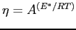
method. Equations 3.1 and 3.2 in their discrete form can be written as:
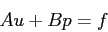 |
(3.5) |
 |
(3.6) |
This system of equations is solved using the Uzawa iteration scheme where at each MG level equation
3.5 is solved iteratively with a Gauss-Seidel method except at the coarsest grid
where it is solved using Conjugate Gradient method and equation 3.6 is applied as a
constraint.
3.4 Test Problems
For the governing equations (3.1-3.4) representing the model problem,
four representative test problems are considered in this section. This selection of test problems,
in two and three dimensions, covers a variety of geodynamical problems related to the Earth's mantle
and lithosphere such as:
- Mantle convection
- Subduction zones
- Mantle plumes
These four representative test problems are described as:
- This "simple 2D test problem" represents time dependent (Rayleigh-Benard) convection with
constant viscosity in a square box
 with temperature fixed to zero at the top, to
 at the bottom and no internal heat source. However, when run for long enough, that is,
thousands of timesteps on a reasonably coarse mesh, and even much more timesteps on a finer mesh,
this will produce a steady-state solution if
at the bottom and no internal heat source. However, when run for long enough, that is,
thousands of timesteps on a reasonably coarse mesh, and even much more timesteps on a finer mesh,
this will produce a steady-state solution if  . It reflects symmetry at the side walls
(i.e.
. It reflects symmetry at the side walls
(i.e.
 ) and zero shear stress on all boundaries of the square box. The Rayleigh
number is
) and zero shear stress on all boundaries of the square box. The Rayleigh
number is
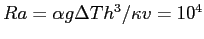 [2] where
  is of
the order of hundreds to thousands of kilometres for mantle convection.
is of
the order of hundreds to thousands of kilometres for mantle convection.
- Time dependent (Rayleigh-Benard) convection with constant viscosity in a unit cube with temperature fixed to zero at the top, to at the bottom and no internal heat
source. However, when run for long enough, that is, thousands of timesteps on a reasonably coarse
mesh, and even much more timesteps on a finer mesh, this will produce a steady-state solution if
. It reflects symmetry at the side walls along the x-direction (i.e.
) and zero shear stress on all boundaries of the unit cube. The Rayleigh number is
[2] where is of the order of hundreds
to thousands of kilometre for mantle convection. This 3D test problem is an extension of the above
simple 2D test problem where a square box is stretched along the y-direction to make it a unit
cube. It is referred to as a ``simple 3D test problem''.
- This "complex 2D test problem" is an extension of the simple 2D test problem and it
represents the important geodynamical process of subduction (where two lithospheres, or plates
meet, and one subducts beneath the other). This extension deals with large and sharp viscosity
contrast. To model this, a temperature-dependent viscosity (with cold material being strong) of
the form
 with
with  the activation energy of mantle material (around 400
kJ/mol), R is the gas constant, and T the absolute temperature.
This viscosity description increases by many (30 or so) orders of magnitude when goes from a
mantle temperature of
the activation energy of mantle material (around 400
kJ/mol), R is the gas constant, and T the absolute temperature.
This viscosity description increases by many (30 or so) orders of magnitude when goes from a
mantle temperature of  down to
  near the surface. As such large viscosity
contrast is impractical to model correctly, the maximum viscosity is cut off to
near the surface. As such large viscosity
contrast is impractical to model correctly, the maximum viscosity is cut off to  times the hot mantle viscosity (the latter being taken as the reference viscosity).
The larger the
times the hot mantle viscosity (the latter being taken as the reference viscosity).
The larger the  -contrast in the calculation, the more difficult for the code to find
convergence for the Stokes equations 3.1 and 3.2. In addition, decoupling
of the two converging plates requires a thin, low viscosity zone. In this test problem, this
low-viscosity zone is set to have a width of tens of kilometres (compared to the full box size of
thousands of kilometres), and has a viscosity similar to that of the hot mantle (even though it
sits within the cold, much stronger lithosphere). This low-viscosity zone and the surrounding
lithosphere form a sharp viscosity contrast.
-contrast in the calculation, the more difficult for the code to find
convergence for the Stokes equations 3.1 and 3.2. In addition, decoupling
of the two converging plates requires a thin, low viscosity zone. In this test problem, this
low-viscosity zone is set to have a width of tens of kilometres (compared to the full box size of
thousands of kilometres), and has a viscosity similar to that of the hot mantle (even though it
sits within the cold, much stronger lithosphere). This low-viscosity zone and the surrounding
lithosphere form a sharp viscosity contrast.
- This "complex 3D test problem" has many of the same features as the complex 2D test
problem. It represents a subduction setting, but one that has ceased to converge (a scenario that
occurs when two continents collide, and neither of them is able to subduct). In this case the
previously subducted lithosphere hangs vertically in the mantle, and eventually breaks off or
diffuses away in the hot mantle. This setup is now modelled in full 3D (which is computationally
more demanding), but doesn't require the weak decoupling zone so that convergence is expected to
be somewhat better.
3.5 Results
This section consists of results for the test problems as described in section
3.4. Each of these test problems is solved using all four multigrid schemes
available at the end of the second phase of this project. The solution times are presented in
seconds for the MG schemes and the number of MPI processes used to get solution in that particular
case. The times for MG schemes and the corresponding number of MPI processes are then presented
graphically followed by plot in log scale to reflect parallel performance and scaling. Further
interpretation of the results is provided with the help of charts representing temperature and
velocity fields. These charts are plotted in the xz-plane for temperature and velocity fields for
test problems in 2D. The same is repeated in the xz-plane and yz-plane for the temperature field and
in the xy-plane and xz-plane for the velocity field, for test problems in 3D.
Solutions for test problems in 2D are obtained for 2, 4, 8, 16, 32 and 64 MPI processes. However,
the quad core configuration of HECToR [9], that is, four cores per node have some
restrictions on fitting the data to the available memory during run time. The available memory
configuration of 8 GB per node or 2 GB per core on HECToR is not sufficient in the case of 2 and 4
MPI process jobs for the 2D test problems under consideration due to the increased size of sub
problem per MPI process. This limits the test runs for 2 MPI process jobs to use one core per node
and test runs for 4 MPI processes jobs to use two cores per node only. In all other cases four cores
per node are used for test problems in 2D. Similarly, solutions for test problems in 3D are
obtained for 32, 64, 128 and 256 MPI processes. Again, the memory configuration of 8 GB per node or
2 GB per core on HECToR is not sufficient in case of 32 and 64 MPI process jobs for the 3D test
problems under consideration due to the increased size of sub problem per MPI process. This limits
the test runs for 32 MPI processes jobs to use one core per node and test runs for 64 MPI processes
jobs to use two cores per node only. In all other cases four cores per node are used for test
problems in 3D.
This way, jobs using one core per node become four times as expensive and jobs using two cores per
node become two times expensive as compared with jobs using four cores per node if the run is for
the same length of time. This encourages us to make better use of compute resources by employing
more MPI processes per node in order to take full advantage of the facility.
Before discussion about the individual test problems and results, it should be noted that first test
problems in 2D and 3D are considered ``simple'' in comparison to the following two test problems
which are considered relatively ``complex''. This comparison is based on the physical nature and the
corresponding computational efforts required for the selected set of test problems. This selection
of test problems is by choice and found to be helpful in identifying strengths and weaknesses of the
MG schemes.
3.5.1 Simple 2D Test Problem
The time taken by each MG scheme to complete 100 timesteps in the case of the simple 2D test problem
is presented in table 3.1. These times are plotted against the number of MPI processes
in figure 3.4 (left) which shows that the V-cycle scheme is performing better when
compared to the other three MG schemes for MPI processes between 2 and 32. The W-cycle scheme
becomes better for 64 MPI processes. However, it is to be noted that performance of FMG(V) and
W-cycle schemes are very close to each other.
Table 3.1:
Time comparison of MG schemes for a simple 2D test problem
| |
Time (in seconds) |
| Number of Processes |
V-cycle |
W-cycle |
FMG(V) |
FMG(W) |
| 2 |
3902 |
4754 |
4487 |
5987 |
| 4 |
1851 |
2264 |
2104 |
2695 |
| 8 |
1026 |
1266 |
1177 |
1515 |
| 16 |
523 |
647 |
613 |
799 |
| 32 |
278 |
354 |
352 |
479 |
| 64 |
182 |
236 |
265 |
384 |
|
Figure 3.4:
Parallel performance and scaling of MG schemes for a simple 2D test problem
|
|
The FMG(W) scheme is slightly more expensive in comparison to the other MG schemes but has the same
pattern. This difference in performance is expected and is due to the nature of this MG
scheme. Further, plots in a log scale 3.4 (right) shows that, apart from small
differences in time, all schemes behave in the same way and scale well up to 32 MPI processes. A
slight deterioration in scaling for 64 MPI processes is noticeable however and it is due to the size
of sub problem which becomes too small for each MPI process, just two elements per MPI process in
any direction, and for this size of sub problem per MPI process, performance and scaling is well
within the acceptable margins.
Figure 3.5:
Temperature and velocity field charts for a simple 2D test problem
|
|
Temperature and velocity fields after the completion of 100 timesteps are shown in figure
3.5. As this is a two dimensional test problem, temperature and velocity fields can
only be drawn in the xz-plane as shown.
3.5.2 Simple 3D Test Problem
This section consists of results for the simple test problem in 3D. As previously mentioned in
section 3.4, this simple test problem in 3D is an extension of the simple test
problem in 2D for which the results and discussion can be found in section 3.5.1.
Table 3.2:
Time comparison of MG schemes for a simple 3D test problem
| |
Time (in seconds) |
| Number of Processes |
V-cycle |
W-cycle |
FMG(V) |
FMG(W) |
| 32 |
21826 |
24656 |
21935 |
25907 |
| 44 |
13548 |
16354 |
13194 |
16736 |
| 128 |
5851 |
6674 |
5869 |
7039 |
| 256 |
3635 |
4420 |
3586 |
4641 |
|
Figure 3.6:
Parallel performance and scaling of MG schemes for a simple 3D test problem
|
|
These results are for between 32 and 256 MPI processes. The time taken by each MG scheme to complete
100 timesteps for this test problem in 3D is presented in table 3.2 and is plotted
against the number of MPI processes in figure 3.6 (left). This graph shows that
V-cycle and FMG(V) schemes perform equally well and slightly better as expected then the
corresponding MG schemes based on the W-cycle, that is, W-cycle and FMG(W) schemes.
The same graph in a log scale 3.6 (right) makes it clear that, apart from negligibly
small differences in time, all schemes behave in the same way and scale well for between 32 and 256
MPI processes. For this test problem in 3D, the sub problem size per process remains of reasonable
size in each case and shows no deterioration in scaling. In other words, all MG schemes scale well
as the number of MPI processes are increased or the sub problem size per MPI process is reduced as
long as it does not become too small as seen in case of simple 2D test problem. However, the
observed bends are thought to be due to the variation in number of cores per node in use for
particular jobs for between 32 and 256 MPI processes.
The temperature and velocity fields after the completion of 100 timesteps are shown in figure
3.7. Due to this being a three dimensional test problem, it is possible to draw these
charts for the temperature field in the yz-plane and the xz-plane and for the velocity field in the
xz-plane and the xy-plane. These charts are drawn at the surface (zero kilometres), at 400 and 800
kilometres away from the surface. As these are drawn just after completion of 100 timesteps, due to
the nature of the test problem, the difference in charts is not easily distinguishable except for
the velocity field charts in the xy-plane.
Figure 3.7:
Temperature and velocity field charts for a simple 3D test problem
|
|
3.5.3 Complex 2D Test Problem
This complex 2D test problem is very difficult to solve numerically and helped in identifying the
weakness of the V-cycle and W-cycle schemes as both of these schemes failed to converge within 12
hours, the maximum allowed time for any job on HECToR. However, FMG(V) and FMG(W) schemes managed to
converge for jobs comprising of between 4 and 64 MPI processes but failed for 2 MPI process jobs.
Table 3.3:
Time comparison of MG schemes for a complex 2D test problem
| |
Time (in seconds) |
| Number of Processes |
V-cycle |
W-cycle |
FMG(V) |
FMG(W) |
| 2 |
- |
- |
* |
* |
| 4 |
- |
- |
22883 |
23238 |
| 8 |
- |
- |
14005 |
18396 |
| 16 |
- |
- |
8934 |
12493 |
| 32 |
- |
- |
5676 |
8286 |
| 64 |
- |
- |
5815 |
7600 |
|
Figure 3.8:
Parallel performance and scaling of MG schemes for a complex 2D test problem
|
|
The time taken by the FMG(V) and FMG(W) MG schemes to complete 100 timesteps in the case of this
complex 2D test problem is presented in table 3.3 and plotted against the number of MPI
processes in figure 3.8 (left) which shows that the FMG(V) scheme is performing better
as compared to the FMG(W) scheme for between 8 and 64 MPI processes. The overall performance pattern
is almost similar in both cases. In particular, performance for 4 MPI process jobs is nearly the
same for both schemes but started deteriorating for 64 MPI process jobs which is acceptable partly
due the decreased sub problem size per MPI process. This deterioration is worse for the FMG(V)
scheme as it took more time for a 64 MPI process job than a 32 MPI process job and is elaborated in
figure 3.8 (right). Apart from this, scaling for up to 32 MPI process jobs is
surprisingly very good for these MG schemes.
Figure 3.9:
Temperature and velocity field charts for a complex 2D test problem
|
|
Temperature and velocity fields after the completion of 100 timesteps are shown in figure
3.9. Due to this being a two dimensional test problem, temperature and velocity fields
are drawn in the xz-plane only. These charts show a sharp change in phase which might be the reason
for the failure of the V-cycle and W-cycle schemes to converge.
3.5.4 Complex 3D Test Problem
This complex 3D test problem is difficult to solve in comparison to the simple 3D test problem but
is relatively easier to solve than the previously attempted complex 2D test problem. This test
problem also helped in identifying some other aspects of the MG schemes.
Table 3.4:
Time comparison of MG schemes for a complex 3D test problem
| |
Time (in seconds) |
| Number of Processes |
V-cycle |
W-cycle |
FMG(V) |
FMG(W) |
| 32 |
42960 |
31386 |
26940 |
34940 |
| 64 |
* |
21205 |
16305 |
22440 |
| 128 |
13167 |
8147 |
7166 |
9306 |
| 256 |
12031 |
5469 |
4423 |
6150 |
|
Time taken by all MG schemes to complete 100 timesteps is presented in table 3.4. It
should be noted that the V-cycle failed to complete 100 timesteps within the permitted maximum time
of 12 hours for any job on HECToR and could complete only 88 timesteps for a 64 MPI process
job. This run was repeated more than once and each time it could only complete 88 timesteps in
contrast to the 32 MPI process job which managed to complete 100 timesteps. This V-cycle scheme
behaviour for 64 MPI process job is neither understood nor logical but found consistent for many
repeated runs.
Figure 3.10:
Parallel performance and scaling of MG schemes for a complex 3D test problem
|
|
These times are plotted against the number of MPI processes in figure 3.10 (left) and
show that the FMG(V) scheme is performing better than any other MG scheme for between 32 and 256 MPI
processes followed by the W-cycle and FMG(W) schemes leaving the V-cycle scheme at the
last. Performance patterns of all schemes are very similar to each other except for the V-cycle
which could not complete 100 timesteps for the 64 MPI process job and started deteriorating for the
256 MPI process job. The other three schemes scale well in contrast to the V-cycle scheme as shown
in figure 3.10 (right). This scaling pattern is very similar to that of MG schemes for
the simple 3D test problem.
Figure 3.11:
Temperature and velocity field charts for a complex 3D test problem
|
|
The temperature and velocity fields after the completion of 100 timesteps are shown in figure
3.11 in the yz-plane and xz-plane for the temperature field and in the xz-plane and
xy-plane for the velocity field. These charts are drawn at the surface (zero kilometres), at 400 and
600 kilometres away from the surface and show changes to the temperature and velocity fields there.
3.5.5 Summary
Analysis of these results for the four representative test problems in the previous sections leads
to a few observations summarised as:
- As a result of this dCSE work, CITCOM performs over 31% faster for the V-cycle multigrid
scheme, over 38% faster for the W-cycle multigrid scheme in comparison to the corresponding
FMG(V) and FMG(W) schemes respectively for the simple 2D test problem and over 12% faster for the
W-cycle multigrid scheme in comparison to the corresponding FMG(W) scheme for the complex 3D test
problem. These figures are based on best performance cases.
- V-cycle scheme is the fastest MG scheme for relatively simple and easy to converge problems.
- FMG schemes perform well in contrast to the corresponding V-cycle and W-cycle schemes for
complex problems. Additionally, later mentioned MG schemes might fail to converge in such cases.
- V-cycle based MG schemes generally perform better than the corresponding W-cycle based MG
schemes
- Scaling of any MG scheme that manages to converge is generally excellent. This is
particularly true if the sub problem size per MPI process is not reduced extremely to the minimum
possible size, that is, just two elements per MPI process in any direction.
- V-cycle scheme offers optimal choice for relatively simple problems and FMG(V) offers optimal
choice for relatively complex problems.
- Scaling might be slightly affected by the use of one or two cores per node in comparison to
the use of all four cores per node.
3.6 Post Processing Tools
This section consists of three types of data processing tools or utilities used in this dCSE project
as described below.
3.6.1 CITCOM Tools
A brief description of CITCOM post processing tools followed by their usage is given below.
3.6.1.1 combcoord
This program/tool combines the local coordinates information from each partition to build the global
coordinates of all nodal points at the finest level of grid.
Syntax of combcoord:
combcoord  inputfile
3.6.1.2 combany
This program/tool combines the first column from files
basename.temp.procID.timestep corresponding to each partition and builds
temperature field corresponding to global node points. In these files, first column contains
temperature field related data.
Syntax of combany:
combany inputfile temp timestep
The argument temp corresponds to the part of the file name containing data, timestep is
the output timestep appended at the end of each output data file name.
3.6.1.3 combvel
This program/tool extracts the velocity field from files
basename.temp.procID.timestep corresponding to each partition and builds
a global velocity field that maps to the global set of nodal points. In these files, columns 2, 3
(in 2D) and 4 (in 3D) represents the x, z, (in 2D) and y (in 3D) components of the velocity field.
Syntax
of combvel:
combvel inputfile timestep
The tools combcoord, combany and combvel use the same order to
store values of coordinates, temperature and velocity fields so that the global nodal points
correspond to these values correctly. The command-line parameters in all these cases have usual
meanings as described:
- inputfile obviously stands for the input file used to run CITCOM job.
- temp is part of the data file name containing the information about a specific field at
node points, e.g. temp stands for temperature field.
- timestep is the interval at which CITCOM writes data to output files.
3.6.1.4 reggrid
This program/tool reads in data processed with combcoord and one of the other two
programs/tools, namely combany or combvel, described above and generates output data
with all necessary information about temperature or velocity for example to be used for drawing
charts as shown in section 3.5
Syntax of reggrid:
reggrid inputfile field snapshot orientation
coordinate discretization discretization
3.6.1.5 regvector
This program/tool does the same job as reggrid except that it adds extra directional arrows
describing the direction of flow for temperature or velocity for example.
Syntax of regvector:
regvector inputfile field snapshot orientation
coordinate discretization vectorscaling
In case of reggrid and regvector, most of the command-line parameters are
similar and can be described as:
- inputfile stands for the input file used to run a CITCOM job.
- field is part of the data file name containing the information about a specific field at
node points, e.g. temp for temperature field.
- snapshot stands for timestep.
- orientation is in x-, z-, or y- coordinate (in 2D or 3D as
appropriate) which is kept fixed, so e.g. y means a plot in xz-plane.
- coordinate is the value of the fixed coordinate, say y 0 or z 100.
It should be noted that in 2D the only possible option for orientation and coordinate is
y 0, that is, a plot in xz-plane only.
- discretization: reggrid allows for separate discretizations in the two
directions of the plane, while regvector uses the same for both; the value is dimensional
and in kilometres.
- vectorscaling is a non-dimensional scaling of the size of vector: the smaller the value,
the smaller the vector sizes. A typical value is 0.001.
3.6.2 Gnuplot
Gnuplot [13] is a copyrighted but freely distributed software, portable and command-line
driven, used for interactive data and function plotting on UNIX, MS Windows, DOS, and many other
platforms. Gnuplot supports many types of plots in 2D and 3D. It can draw using lines, points,
boxes, contours, vector fields, surfaces, and various associated text. It also supports various
specialised plot types.
Gnuplot supports many different types of output: interactive screen terminals, direct output to pen
plotters or modern printers, and output to many file formats, for example, eps, fig, jpeg, LaTeX,
metafont, pbm, pdf, png, postscript, svg, etc.
All graphs presented in this report in section 3.5 are drawn using Gnuplot.
3.6.3 The Generic Mapping Tools (GMT)
The Generic Mapping Tools or GMT [14] is an open source collection of more than 60 programs
for manipulating geographic and Cartesian data sets including filtering, trend fitting, gridding,
projecting, etc. and producing (encapsulated) postscript file illustrations ranging from simple
xy plots via contour maps to artificially illuminated surfaces and 3D perspective
views. GMT supports nearly 30 map projections and transformations and comes with a variety of
support data. Charts given in section 3.5 are generated using a few of the GMT components
which are described in table 3.5.
Table 3.5:
GMT programs and their description.
| Program |
Description |
| grdcontour |
Contouring of 2-D gridded data sets |
| grdimage |
Produce images from 2-D gridded data sets |
| makecpt |
Make color palette tables |
| psbasemap |
Create a basemap plot |
| psscale |
Plot gray scale or colour scale on maps |
| xyz2grd |
Convert an equidistant table xyz file to a 2-D grid file |
|
3.7 Next Phase
Next phase (phase 3) of this dCSE project consists of two tasks:
- Mesh refinement near high viscosity gradients.
- Improved prolongation and restriction
These tasks are explained briefly along with some questions on implementation feasibility within
CITCOM code structure.
3.7.1 Mesh Refinement
Mesh refinement in MG methods is clearly distinct from the common procedure of smoothly decreasing
the element size towards the location where velocity or viscosity gradients are large. Such a method
is very difficult to combine with a structured mesh that requires a nested set of MG
meshes. However, MG naturally offers a different local mesh refinement method. By locally adding one
or more finer layers, the resolution can locally be improved by a factor of  or powers of
. One such possible scenario of uniform local refinement is depicted in figure
3.12(left) where only the boundary elements are refined.
or powers of
. One such possible scenario of uniform local refinement is depicted in figure
3.12(left) where only the boundary elements are refined.
Figure 3.12:
Examples of uniform (left) and non-uniform (right) refinement
|
|
The other scenario of non-uniform local refinement which is more complicated and difficult to
implement is depicted in figure 3.12(right). Since the grid elements at the
finer MG levels do not exist globally, these levels require some special treatment, and introduce
some complexity to the solution methods as well. In order to handle this complexity there might be a
need to introduce an extra layer of ``ghost nodal points'' on the interior boundaries and/or extra
bookkeeping of the information at the finer grid levels which do not exist everywhere. This would
increase memory requirements significantly and lead to load imbalance in most cases.
Due to importance of the local mesh refinement and the envisaged improvement it can make to the rate
of convergence, the implementation of this scenario is the top priority in the next phase.
3.7.2 Improvements to Prolongation and Restriction
Restriction and prolongation operations may help to improve the rate of convergence by adopting
different averaging schemes [1] as suggested in the proposal. However, studying the
current implementations for restriction (based on weighted averaging) and prolongation (based on
weighted interpolation), previous experience of the PI and outcome of the discussion with the PI on
this topic suggests that it is highly unlikely to gain any significant advantage by implementing
suggested averaging schemes over the existing implementation.
Therefore it is agreed that the work in phase 3 would concentrate on the implementation of the local
mesh refinement.
Next: 4. Refinement
Up: Multigrid Improvements to CITCOM
Previous: 2. Initial Project Study
Contents
Sarfraz A Nadeem
2010-06-15
![\includegraphics[width=75mm,height=56mm]{figures/v-cycle.eps}](img12.png)
![\includegraphics[width=75mm,height=56mm]{figures/w-cycle.eps}](img13.png)
![\includegraphics[width=95mm,height=56mm]{figures/fmg-cycle.eps}](img14.png)
![\fbox{
\includegraphics[width=60mm,height=45mm]{graphs/bb2d.eps}\hspace{6mm}
\includegraphics[width=60mm,height=45mm]{graphs/bb2d-log.eps}
}](img43.png)
![\fbox{
\includegraphics[width=60mm,height=45mm]{charts/bb2dBV032.temp_y0.100.ep...
...m}
\includegraphics[width=60mm,height=45mm]{charts/bb2dBV032.vel_y0.100.eps}
}](img44.png)
![\fbox{
\includegraphics[width=60mm,height=45mm]{graphs/bb3d.eps}\hspace{6mm}
\includegraphics[width=60mm,height=45mm]{graphs/bb3d-log.eps}
}](img45.png)
![\includegraphics[width=40mm,height=30mm]{charts/bb3dFV032.temp_x0.100.eps}](img46.png)
![\includegraphics[width=40mm,height=30mm]{charts/bb3dFV032.temp_x400.100.eps}](img47.png)
![\includegraphics[width=40mm,height=30mm]{charts/bb3dFV032.temp_x800.100.eps}](img48.png)
![\includegraphics[width=40mm,height=30mm]{charts/bb3dFV032.temp_y0.100.eps}](img49.png)
![\includegraphics[width=40mm,height=30mm]{charts/bb3dFV032.temp_y400.100.eps}](img50.png)
![\includegraphics[width=40mm,height=30mm]{charts/bb3dFV032.temp_y800.100.eps}](img51.png)
![\includegraphics[width=40mm,height=30mm]{charts/bb3dFV032.vel_y0.100.eps}](img52.png)
![\includegraphics[width=40mm,height=30mm]{charts/bb3dFV032.vel_y400.100.eps}](img53.png)
![\includegraphics[width=40mm,height=30mm]{charts/bb3dFV032.vel_y800.100.eps}](img54.png)
![\includegraphics[width=40mm,height=30mm]{charts/bb3dFV032.vel_z0.100.eps}](img55.png)
![\includegraphics[width=40mm,height=30mm]{charts/bb3dFV032.vel_z400.100.eps}](img56.png)
![\includegraphics[width=40mm,height=30mm]{charts/bb3dFV032.vel_z800.100.eps}](img57.png)
![\fbox{
\includegraphics[width=60mm,height=45mm]{graphs/bp2d.eps}\hspace{6mm}
\includegraphics[width=60mm,height=45mm]{graphs/bp2d-log.eps}
}](img58.png)
![\fbox{
\includegraphics[width=60mm,height=45mm]{charts/bp2dFV032.temp_y0.100.ep...
...m}
\includegraphics[width=60mm,height=45mm]{charts/bp2dFV032.vel_y0.100.eps}
}](img59.png)
![\fbox{
\includegraphics[width=60mm,height=45mm]{graphs/bar3d.eps}\hspace{6mm}
\includegraphics[width=60mm,height=45mm]{graphs/bar3d-log.eps}
}](img60.png)
![\includegraphics[width=40mm,height=30mm]{charts/bar3dFV032.temp_x0.100.eps}](img61.png)
![\includegraphics[width=40mm,height=30mm]{charts/bar3dFV032.temp_x400.100.eps}](img62.png)
![\includegraphics[width=40mm,height=30mm]{charts/bar3dFV032.temp_x800.100.eps}](img63.png)
![\includegraphics[width=40mm,height=30mm]{charts/bar3dFV032.temp_y0.100.eps}](img64.png)
![\includegraphics[width=40mm,height=30mm]{charts/bar3dFV032.temp_y400.100.eps}](img65.png)
![\includegraphics[width=40mm,height=30mm]{charts/bar3dFV032.temp_y800.100.eps}](img66.png)
![\includegraphics[width=40mm,height=30mm]{charts/bar3dFV032.vel_y0.100.eps}](img67.png)
![\includegraphics[width=40mm,height=30mm]{charts/bar3dFV032.vel_y400.100.eps}](img68.png)
![\includegraphics[width=40mm,height=30mm]{charts/bar3dFV032.vel_y800.100.eps}](img69.png)
![\includegraphics[width=40mm,height=30mm]{charts/bar3dFV032.vel_z0.100.eps}](img70.png)
![\includegraphics[width=40mm,height=30mm]{charts/bar3dFV032.vel_z400.100.eps}](img71.png)
![\includegraphics[width=40mm,height=30mm]{charts/bar3dFV032.vel_z600.100.eps}](img72.png)
![\includegraphics[width=65mm,height=65mm]{pictures/localrefinement.eps}](img76.png)
![\includegraphics[width=65mm]{pictures/nonuniformrefinement.eps}](img77.png)