Proposed Eigensolver

Consider the following:

$$\hat{H}\psi_i = \epsilon_i \hat{S}\psi_i$$

$$\Rightarrow \left(\hat{H}-\lambda\hat{S}\right) \psi_i = \left(\epsilon_i-\lambda\right) \hat{S}\psi_i$$

$$\Rightarrow \left(\hat{H}-\lambda\hat{S}\right)^\dagger\left(\hat{H}-\lambda\hat{S}\right) \psi_i = \left(\epsilon_i-\lambda\right)^2 \hat{S}\psi_i$$ (6.4)

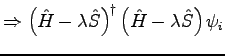
Equation 6.4 is simply a modified eigenvalue equation that shares the same eigenstates as the original Schrödinger-like equation but with modified eigenvalues. However the lowest eigenvalue of this modified equation is not the lowest energy eigenvalue $\epsilon_0$, but the eigenstate whose eigenvalue is closest to $\lambda$. Furthermore, the eigenstate with eigenvalue $\lambda$ is now at a local minimum, regardless of whether it has the globally lowest eigenvalue or not.

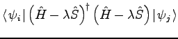
Consider now the usual Castep algorithm outlined in section 6.2, for the special case where each block contains only a single eigenstate. If we omit the orthonormalisation step then every approximate eigenstate will tend to converge to the lowest eigenstate, but if we first replace the augmented subspace matrix

$$H_{ij} = \ensuremath{\left \langle \left. \psi_i \right. \right\vert \hat{H} \left\vert \left. \psi_j \right. \right \rangle}$$ (6.5)

with the modified matrix,

$$M_{ij} = \ensuremath{\left \langle \left. \psi_i \right. \right\vert \left... ...(\hat{H}-\lambda\hat{S}\right) \left\vert \left. \psi_j \right. \right \rangle}$$

$$= \ensuremath{\left\langle \left. \left(\hat{H}-\lambda\hat{S}\righ... ...ht. \right\vert \left. \left(\hat{H}-\lambda\hat{S}\right)\psi_j \right\rangle}$$

then by varying the value of $\lambda$ we can select which of the modified eigenvalues is lowest.

If we choose $\lambda=\epsilon_i$ then this algorithm will automatically choose the best approximate eigenstate closest to the initial approximation. In this case the states in the inner product are the band residuals $R$,

$$R_i = \hat{H}\psi_i - \epsilon_i\hat{S}\psi_i$$ (6.6)

and the algorithm is very similar to the Residual Minimisation Method by Direct Inversion in an Iterative Subspace algorithm (RMM-DIIS)[3].

The only difference between our scheme and the usual RMM-DIIS method is the choice of state to add to our block's subspace. In the usual Castep scheme we add a state $\phi$ given by

$$\phi = \hat{K}\left(\hat{H}\psi_i-\epsilon_i\hat{S}\psi_i\right).$$ (6.7)

In the RMM-DIIS scheme we search along this direction for the minimal residual norm, i.e. find a new trial eigenstate along the direction $\phi$, and add that trial eigenstate to the subspace instead of $\phi$. The schemes are so similar that we implemented both in Castep.

After all of the eigenstates have been updated, a global orthonormalisation is still necessary before a new density can be constructed. However this single orthonormalisation per SCF cycles is considerably fewer than the usual Castep scheme where three or four orthonormalisations are per SCF cycle are common.

Both schemes converge to the closest eigenstate to the current trial eigenstate, so it is important that we have a reasonable set of trial eigenstates before using these schemes. We opted to use the usual Castep optimisation for four SCF cycles before switching to one of the new schemes.