The structure constants were stored in a 4 index fortran array
![]() . This way the atom pair with the largest
. This way the atom pair with the largest ![]() block defines the memory requirements which may be of substantial size since the maximal
block defines the memory requirements which may be of substantial size since the maximal
![]() , in this case
may reach
, in this case
may reach ![]() , as used in the basis
functions for the operators and
, as used in the basis
functions for the operators and ![]() , for when forces or pressure also needs to be calculated in the end of the last self-consistency
iteration. For example, a
, for when forces or pressure also needs to be calculated in the end of the last self-consistency
iteration. For example, a ![]() element like Ti is given up to a
element like Ti is given up to a ![]() orbital
orbital ![]() resulting in structure block size for the pair Ti-
Ti of up to
resulting in structure block size for the pair Ti-
Ti of up to
![]() compared with
compared with
![]() for a Hamiltonian
block. To reduce the memory requirements the original implementation exploited two symmetry properties:
for a Hamiltonian
block. To reduce the memory requirements the original implementation exploited two symmetry properties:
![]() and
and
![]() .
.
The second rule means that the extra ![]() part may be calculated only once then obtained from this for the reverse pair.
The calculation of a single block consists of first evaluating the Hankel functions for
part may be calculated only once then obtained from this for the reverse pair.
The calculation of a single block consists of first evaluating the Hankel functions for
![]() then calculating a dot product over
then calculating a dot product over ![]() with the Gaunt coefficients stored in packed format.
The Hankel function is directly computed for a non periodic case while Ewald summation is performed in the periodic case.
This is the slowest part of the calculation.
with the Gaunt coefficients stored in packed format.
The Hankel function is directly computed for a non periodic case while Ewald summation is performed in the periodic case.
This is the slowest part of the calculation.
The electrostatic potential calculation computation consists of a matrix by block vector product between
the structure constants and the charge multipoles along the ![]() indices. A convenient optimisation is to swap the
indices, resulting in
indices. A convenient optimisation is to swap the
indices, resulting in
![]() and then spread the
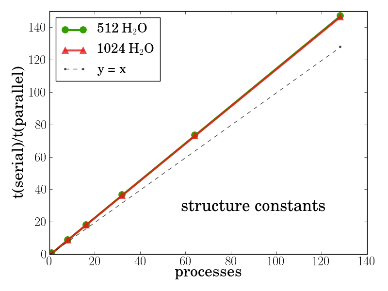
and then spread the ![]() atoms over all available processes as evenly as possible
without splitting a block to avoid doubling of the effort for the Hankels. In this way the storage is distributed
over the processes and only a small gather operation for the final potential block vector is needed.
This strategy was implemented and showed superlinear performance which is most likely due to the decreased memory
requirements per process, see Fig 4.
atoms over all available processes as evenly as possible
without splitting a block to avoid doubling of the effort for the Hankels. In this way the storage is distributed
over the processes and only a small gather operation for the final potential block vector is needed.
This strategy was implemented and showed superlinear performance which is most likely due to the decreased memory
requirements per process, see Fig 4.
Since often one needs to study systems containing atoms of different type e.g. H2O, Ti2O, etc., the pair with lower ![]() requirements waste a significant portion of the allocated block size. For example in a H2O molecule we would allocate
requirements waste a significant portion of the allocated block size. For example in a H2O molecule we would allocate
![]() KB and only use
KB and only use
![]() KB.
The difference is striking
and for this reason the fixed block format was abandoned. Having the block structure however is more convenient and cache
friendly than dealing with the normal array so the solution was to create an index of pointers and preserve the storage format
while achieving a fivefold decrease the total memory requirements. This was actually a second revision due to difficulty
interfacing the first implementation, which was based on a 2D Fortran pointer array with C/CUDA.
KB.
The difference is striking
and for this reason the fixed block format was abandoned. Having the block structure however is more convenient and cache
friendly than dealing with the normal array so the solution was to create an index of pointers and preserve the storage format
while achieving a fivefold decrease the total memory requirements. This was actually a second revision due to difficulty
interfacing the first implementation, which was based on a 2D Fortran pointer array with C/CUDA.