This report documents the work performed during the dCSE
project titled “Improved Data Distribution Routines for Gyrokinetic Plasma
Simulations”. The project, undertaken at
EPCC, The University of Edinburgh, in conjunction with CCFE at Culham, aimed to
improve the overall performance of the GS2 code, thereby reducing the
computational resources required to undertake scientific simulations, enabling
more efficient use of the resources provided by the HECToR service (and other
HPC systems).
GS2 is an
initial value simulation code developed to study low-frequency turbulence in
magnetized plasma. GS2 solves the gyrokinetic equations for perturbed
distribution functions together with Maxwell’s equations for the turbulent
electric and magnetic fields within a plasma.
It is typically used to assess the microstability of plasmas produced in
the laboratory and to calculate key properties of the turbulence which results
from instabilities. It is also used to simulate turbulence in plasmas which
occur in nature, such as in astrophysical and magnetospheric systems.
Gyrokinetic
simulations solve the time evolution of the distribution functions of each
charged particle species in the plasma, taking into account the charged
particle motion in self-consistent magnetic and electric fields. These
calculations are undertaken in a five dimensional data space, with three
dimensions for the physical location of particles and two dimensions for the
velocity of particles. More complete six dimensional kinetic plasma
calculations (with three velocity space dimensions) are extremely time
consuming (and therefore computational very costly) because of the very rapid
gyration of particles under the strong magnetic fields. Gyrokinetic simulations simplify this six
dimensional data space by averaging over the rapid gyration of particles around
magnetic field lines and therefore reducing the problem from six to five dimensions (where velocity is
represented by energy and pitch angle, and the gyrophase angle is averaged
out). While the fast gyration of particles is not calculated in full, it is
included in a gyro-averaged sense allowing lower frequency perturbations to be
simulated faithfully at lower computational cost.
GS2 can be used
in a number of different ways, including linear microstability simulations,
where growth rates are calculated on a wavenumber-by-wavenumber basis with an
implicit initial-value algorithm in the ballooning (or "flux-tube")
limit. Linear and quasilinear properties of the fastest growing (or least
damped) eigenmode at a given wavenumber may be calculated independently (and
therefore reasonably quickly). It can
also undertake non-linear gyrokinetic simulations of fully developed
turbulence. All plasma species
(electrons and various ion species) can be treated on an equal, gyrokinetic
footing. Nonlinear simulations provide fluctuation spectra, anomalous
(turbulent) heating rates, and species-by-species anomalous transport
coefficients for particles, momentum, and energy. However, full nonlinear simulations are very
computationally intensive so generally require parallel computing to complete
in a manageable time.
GS2 is a fully
parallelised, open source, code written in Fortran90. The parallelisation is implemented with MPI,
with the work of a simulation in GS2 being split up (decomposed) by assigning
different parts of the distribution functions to different processes to
complete.
For any given
GS2 input file (which specifies the simulation to be carried out, including the
domain decomposition layout) the program ingen
provides a list of recommended process counts (or “sweet spots”) for the GS2
simulation to be run on, along with some other useful information on the
simulation parameters provided by the user. These recommendations are
calculated from the properties prescribed in the input file of the simulation
to be run, and aim to split the data domain as evenly as possible to achieve
good “load-balancing” (which helps to optimise the performance of the program
and minimise the runtime). The primary
list of recommended process counts is based on the main data layout, g_lo,
that is used for the linear parts of the simulations. ingen
also provides lists of process counts that are suitable for the nonlinear parts
of the calculations (referred to as xxf_lo
and yxf_lo process counts) which
may differ from the process counts recommended for g_lo.
For optimal
performance with GS2, choosing a process count that is in all three of the
lists of process counts that ingen
provides is beneficial. However, this is
not always possible, especially at larger process counts, and in this scenario
users generally choose a process count that is optimal for g_lo.
HECToR[7], a Cray
XE6 computer, is the UK National Supercomputing Service. This project utilised both the Phase 2b and
Phase 3 phases of the system. Phase 2b
XE6 system consisted of 1856 compute nodes, each containing two 2.1 GHz 12-core
‘Magny-cours’ AMD Opteron processor and 32 GB of main memory, giving 1.33 GB
per core. The nodes were coupled with
Cray’s Gemini network, providing a high bandwidth and low latency 3D torus
network. The peak performance of the system was 360 TFlops, and ranked 16th in
the June 2010 Top 500 list.
Phase 3, the
current incarnation of HECToR, uses two 16-core 2.3 GHz ’Interlagos’ AMD
Opteron processors per node, giving a total of 32 cores per node, with 1 GB of
memory per core. The addition of 10 cabinets (928 compute nodes) to the Phase
2b configuration increased the peak performance of the whole system to over 820
TF.
This DCSE project follows up on findings from a previous GS2
DCSE project (“Upgrading
the FFTs in GS2”) that was carried out by EPCC in 2010. The goal of that project was to implement
FFTW3 functionality and optimise the FFTs used by GS2. During this work it was discovered that the
GS2 code to transform data between layouts associated with the FFTs was consuming a large fraction of the
runtime.
Specifically, the routines c_redist_22
and c_redist_32 were highlighted
as being costly, with about 8% of runtime being spent on each (for a benchmark
run on 1024 cores). These routines redistribute/rearrange data from xxf_lo to yxf_lo, and from g_lo
to xxf_lo, respectively, as
required for performing FFTs. This requires coordinating data to be communicated
to or received from other processes, and rearranging the data that is available
locally. These routines make extensive
use of indirect addressing when packing the buffers.
Indirect addressing is a form of array access where the
indices of the array being accessed are themselves stored in a separate
array. Here is an example of a standard
FORTRAN array access:
to_here(i, j) = from_here(i, j, k) code I
Similar array copying code is used in these GS2 routines,
but making extensive use of indirect addressing like this:
to_here(to_index(i)%i, to_index(i)%j) = from_here(from_index(i)%i, from_index(i)%j, code II
from_index(i)%k)
Whilst such functionality is very useful in providing a
simple standard interface for a program to access data stored in an array in a
variety of different layout patterns (indeed this allows GS2 to rearrange data
layouts without having to change any array index code at the point of use) and
was common in codes exploiting vector architectures, this functionality does introduce
additional computational costs, and in particular the memory access cost of
this array transformation on modern computing hardware increases significantly.
In the traditional example (code I) the code requires one memory load (from_here(i, j, k)) and one memory store (to_here(i, j)) (assuming the indexes i, j,
and k are stored in cache or
registers on the processor). With the
indirect addressing functionality (code II) six memory loads are required (one
for each index look-up and one to retrieve the data in from_here) and one memory store. Given that undertaking memory operations is
very costly on a modern processor (compared to performing computation), and
given that accesses like these take a significant part of the routines highlighted
as being costly in GS2, this is evidently impacting performance.
In this report we:
- outline
the current redistribution and indirect addressing functionality and
document its performance
- describe
our approach for optimising the indirect addressing code and assess the
performance impact of these optimisations.
- discuss
the data decompositions used by GS2 and how these can be optimised further
- describe
the functionality that is currently used for copying data between
processes and our attempts to optimise it.
GS2 supports
six different data layouts for the g_lo
datatype array containing the perturbed distribution functions for all the
plasma species. These layouts are: ”xyles”,
”yxles”, “lyxes”, “yxels”,
“lxyes”, “lexys”. The layout can be chosen at run time by the user
(through the input parameter file).
Each character
in the layout represents a dimension in the simulation domain as follows (the
name in brackets is the variable name used for the dimension in the code)
·
x: Fourier wavenumber in X (ntheta0)
·
y: Fourier wavenumber in Y (naky)
·
l: Pitch angle (nlambda)
·
e: Energy (negrid)
·
s: Particle species (nspec)
The layout controls how the data domain in GS2 is
distributed across the processes in the parallel program, controlling the order
in which individual dimensions in the data domain iterate in the compound index
that will be distributed (split up)
across the processes. For instance, in
the “”xyles” layout
the species index, “s”, iterates
most slowly, and “x” iterates
most rapidly, whereas in the “lexys” “s” iterates most slowly and the pitch angle index, “l”, iterates
most rapidly..
Linear
calculations with GS2 are performed in k-space using the g_lo layout as this is computationally
efficient. The nonlinear terms, however,
are more efficiently calculated in position space. Therefore, when GS2 undertakes a nonlinear
simulation, it computes the linear advance in k-space, and the nonlinear
advance in position space. While the majority of the simulation is in k-space,
each timestep there are FFTs into position space, to evaluate the nonlinear
term, and an inverse FFT to return the result into k-space. Whilst users need not concern themselves with
these implementation details, this use of both k- and position space can impact
on performance, depending on the number of processes used in the parallel
computation.
In the linear
part of calculations GS2's distribution functions are parallelised in k-space,
using the GS2 g_lo data layout.
The non-linear parts of calculations, which require FFTs, use two different
data distribution layouts, namely xxf_lo and yxf_lo. These are
required for the two stages (one for 1D FFTs in x,
the other for 1D FFTs in y)of
each of the forward and inverse FFTs
Practically the GS2
data space is stored in a single array, but it can be considered conceptually
as a 7 dimensional data object. Five of the dimensions are the previously
discussed x,y,l,e,s, the other two
are ig (the index corresponding to the spatial
direction parallel to the magnetic field) and isgn (isgn corresponds to the
direction of particle motion in the direction parallel to the magnetic field, b; for GS2 isgn =1
represents particles moving parallel to b,
and isgn=2 represents particles moving antiparallel to
b). In this report we study the
following three distribution layouts of the distribution function in GS2:
- g_lo(ig,isgn:”layout”): indices ig and isgn are guaranteed
to be kept local to each process, and x,y,l,e,s are decomposed (with the decomposition
depending on the chosen “layout”).
- xxf_lo(ix:iy,ig,isgn,”les” data space only ix is guaranteed to be kept local, and
the compound index includes iy,ig,isgn,l,e,s (where y is the fastest index and the order of l,e,s
depends on the chosen “layout”).
- yxf_lo(iy:ix,ig,isgn,”les”) data space only iy is kept local and the compound index
contains ix,ig,isgn,l,e,s
(where ix is the fastest
index and the order of “les” depends on the chosen “layout”).
GS2 uses a
dealiasing algorithm to filter out high wavenumbers in X and Y,
which is a standard technique to avoid non-linear numerical instabilities in
spectral codes. g_lo contains the filtered
data, which has lower ranges of indices in X and Y than in the xxf_lo and yxf_lo layouts. This means that after the yxf_lo stage the amount of data is larger than at the g_lo stage (approximately 2¼ times
larger).
The functions we have considered for optimisation are the
routines c_redist_22 and c_redist_32 and their inverse versions
c_redist_22_inv and c_redist_32_inv, which perform the data transformations
required for the FFTs. The evaluation
of each 2D FFT requires transformations,
or redistributions, to be undertaken in two phases. Firstly, c_redist_32
transforms the data from the three index g_lo
data structure into the two index data structure xxf_lo
which is used for the first FFT in x. Later c_redist_22
performs the additional transpose required for the FFT in y, converting from the intermediate xxf_lo data structure to the yxf_lo
layout. After the computation of the
nonlinear terms in real space, the transformations and FFTs must be performed
in reverse using the _inv
routines to obtain the nonlinear term in k-space.
Within the redistribution routines there are two types of
functionality, to perform local and remote copies. The local copy redistributes any data which
will belong to the same process in both data layouts, and remote copy
redistributes the data that must be communicated between different processes (including collecting the data to
be sent to each process in a buffer, sending the data to that process, and
unpacking all received data into the local data array).
Initial benchmarking of the code using a representative
benchmark case (see the GS2 input file in appendix A) produced the following
performance figures on HECToR Phase2b (where the times are seconds):
|
Number of Cores:
|
128
|
256
|
512
|
1024
|
|
c_redist_22
|
Local Copy
|
53.71
|
27.17
|
13.73
|
6.81
|
|
|
Remote Copy
|
0.07
|
0.13
|
0.26
|
0.48
|
|
c_redist_22_inv
|
Local Copy
|
13.73
|
6.90
|
3.46
|
1.76
|
|
|
Remote Copy
|
0.01
|
0.03
|
0.05
|
0.10
|
|
c_redist_32
|
Local Copy
|
49.85
|
25.60
|
12.46
|
3.92
|
|
|
Remote Copy
|
0.05
|
0.10
|
0.19
|
9.22
|
|
c_redist_32_inv
|
Local Copy
|
12.31
|
6.26
|
2.79
|
0.77
|
|
|
Remote Copy
|
0.01
|
0.03
|
0.05
|
1.99
|
Table 1:
Initial Benchmarking of the redistribution functionality (using the “xyles”
layout and running for 500 iterations)
These results showed that:
·
Local copy parts of the routine dominate
performance of those routines for lower core counts.
·
At larger processor/core counts, e.g. 1024
cores, the remote copy functionality significantly affects performance,
especially for c_redist_32.
In section 3 we
describe our efforts to optimise the local copy parts of these routines by
replacing the currently implemented indirect addressing functionality. Section 4 outlines our approaches at
optimisation of the remote copy code by introducing non-blocking communications
and by replacing some of the indirect addressing functionality. Section 5 describes further optimisations of
the data decompositions used in GS2.
As previously discussed indirect addressing, where the
indexes used to access an array of data are themselves stored in a separate
array, is heavily used in GS2 to perform the data redistributions required to
undertake the 2D FFTs that compute the nonlinear terms. As indirect addressing can be costly, both in
terms of the impact on computational time and memory consumption, we looked to
replace this functionality with a more direct approach to improve the
performance of the local copy parts of GS2.
The next subsection outlines the original functionality in the code. The
subsections that follow outline our new optimised code and the performance
improvements that were achieved.
The indirect addresses used in the redistribution in GS2 are
constructed using the following code (in the source file gs2_transforms.fpp):
Indirect addresses for the _22
routines (in subroutine init_y_redist):
do
ixxf
=
xxf_lo%llim_world,
xxf_lo%ulim_world
do it
=
1,
yxf_lo%nx
call xxfidx2yxfidx
(it,
ixxf,
xxf_lo,
yxf_lo,
ik,
iyxf)
if (idx_local(xxf_lo,ixxf))
then
ip =
proc_id(yxf_lo,iyxf)
n =
nn_from(ip)
+
1
nn_from(ip) =
n
from_list(ip)%first(n) =
it
from_list(ip)%second(n)
=
ixxf
end if
if (idx_local(yxf_lo,iyxf))
then
ip =
proc_id(xxf_lo,ixxf)
n =
nn_to(ip)
+
1
nn_to(ip) =
n
to_list(ip)%first(n) =
ik
to_list(ip)%second(n) =
iyxf
end if
end do
end
do
Indirect address for the _32
routines (in subroutine init_x_redist):
do
iglo
=
g_lo%llim_world,
g_lo%ulim_world
do
isign
=
1,
2
do
ig
=
-ntgrid,
ntgrid
call
gidx2xxfidx
(ig,
isign,
iglo,
g_lo,
xxf_lo,
it,
ixxf)
if
(idx_local(g_lo,iglo))
then
ip =
proc_id(xxf_lo,ixxf)
n =
nn_from(ip)
+
1
nn_from(ip) =
n
from_list(ip)%first(n) =
ig
from_list(ip)%second(n)
=
isign
from_list(ip)%third(n) =
iglo
end
if
if
(idx_local(xxf_lo,ixxf))
then
ip =
proc_id(g_lo,iglo)
n =
nn_to(ip)
+
1
nn_to(ip) =
n
to_list(ip)%first(n) =
it
to_list(ip)%second(n) =
ixxf
end
if
end
do
end
do
end
do
The from_list
and to_list data structures are
created on initialisation for each of the xxf_lo
and yxf_lo data formats (where
they are called to and from rather than to_list and from_list), and are dynamically allocated for each
process by iterating through the whole data space and calculating which indexes
will be sent from and received by a given process.
We can see from the
above functionality that the to
and from address lists are
constructed together, but using different functionality. In both cases there is a loop across the full
set of points defined by the lower and upper bounds xxf_lo%llim_world and xxf_lo%ulim_world. These variables store the lower and upper
bounds of the compound index in the xxf_lo data structure, which are the same
for all processes and defined within a function called init_x_transform_layouts (in the file gs2_layouts.fpp) as follows:
xxf_lo%llim_world
=
0
xxf_lo%ulim_world
=
naky*(2*ntgrid+1)*2*nlambda*negrid*nspec
-
1
The parameters
used in the calculation of xxf_lo%ulim_world
are defined in the GS2 input file. The
inner loops do not change their bounds for the iterations of the outer loop and
are also the same for all processes.
Within the main loops there is a
function call and then two if
branches: one to set the indices for the to
array; and the other to set the indices for the from
array. The indices are assigned as
elements of the to_list(ip)%first
and to_list(ip)%second arrays, with each process in the program
having these arrays pointing to different ranges of indices (i.e. if we look at
to_list(ip)%first(n) the
ip represents a particular process
number and the n represents how
many entries for this processor have currently been assigned).
The indirect addresses constructed here in the from_list and to_list
variables are then stored as a redist_type
variable r via a call to the init_redist subroutine (in redistribute.f90).
These indirect addresses are then used in c_redist_22 routine as follows
(contained within source file utils/redistributed.f90):
do i = 1, r%from(iproc)%nn
to_here(r%to(iproc)%k(i), &
r%to(iproc)%l(i)) &
= from_here(r%from(iproc)%k(i), &
r%from(iproc)%l(i))
end do
c_redist_32 is
similar, but with the added complication that it reduces 3 indices to 2 indices
in the copy:
do i = 1, r%from(iproc)%nn
to_here(r%to(iproc)%k(i),&
r%to(iproc)%l(i)) &
= from_here(r%from(iproc)%k(i), &
r%from(iproc)%l(i), &
r%from(iproc)%m(i))
end do
A more optimal loop for c_redist_22, with a rather more efficient structure, would be the following:
do i = 1, upperi
do j = 1, upperj
to_here(i,j) = from_here(i,j)
end do
end do
Such a structure requires only one memory load (the from_here(i,j) part), one memory store (for the to_here(i,j) part), a counter increment (do j),
and a loop counter comparison for each loop operation. This would be much more efficient than the c_redist_22 loop which performs five memory loads and
one memory store plus one loop increment and one loop counter comparison. This, along with the possibility for enabling
better cache re-use (based on spatial or temporal locality), shows the
potential for optimising these loops by replacing the indirect addressing with
direct addressing.
In optimising the implementation for local copies, we exploited the fact that the
indirect addresses from_list and
to_list (constructed as described in Section 3.1) have their indices set to the same value (ip=iproc).
- in c_redist_22 this
restricts the values of interest in
the ixxf and it loops to where iproc == iyxf/yxf_lo%blocksize == ixxf/xxf_lo%blocksize.
- in c_redist_32 this
constraint restricts the values of interest in the iglo, isgn, and ig loops to where iproc == iglo/g_lo%blocksize and iproc == ixxf/xxf_lo%blocksize.
With these equalities we can reduce the use of
indirect addressing by using an initial ixxf
or iglo value (provided by the existing to and from
arrays already calculated in the code), and working through the existing loops
(the it
loop for c_redist_22 and the ik and iyxf
loops for c_redist_32) using the
simple rules that are currently used with those loops.
The only other functionality required is loop termination,
or upper bounds, to enable proper termination of the loops in the situation
where the theoretical data space for processes is larger than the actual data
space assigned to each process (this is dealt with in the existing indirect
addressing code by comparing computed indices with the appropriate %ulim_proc values, and this is what we
do as well).
Using these
different functional aspects it was possible to construct the following
replacement code for the c_redist_22 local copy functionality:
i = 1
do while (i .le. r%from(iproc)%nn)
itmin = r%from(iproc)%k(i)
ixxf = r%from(iproc)%l(i)
ik = r%to(iproc)%k(i)
iyxf = r%to(iproc)%l(i)
it_nlocal = (yxf_lo%ulim_proc+1) - iyxf
itmax = min((itmin-1)+it_nlocal,yxf_lo%nx)
do it = itmin,itmax
to_here(ik,iyxf) = from_here(it,ixxf)
iyxf = iyxf + 1
i = i + 1
end do
end do
And likewise for the
c_redist_32 local copy functionality the following code
can be constructed that removes most of the original indirect addressing
functionality:
i = 1
nakyrecip = naky
nakyrecip = 1/nakyrecip
f2max = r%from_high(2)
do while(i .le. r%from(iproc)%nn)
f2 = r%from(iproc)%l(i)
f3 = r%from(iproc)%m(i)
t1 = r%to(iproc)%k(i)
do while (f2 .le. f2max)
f1 = r%from(iproc)%k(i)
t2 = r%to(iproc)%l(i)
thigh = ceiling(((xxf_lo%ulim_proc+1) - t2)*nakyrecip)
thigh = thigh + (f1-1)
fhigh = min(thigh,r%from_high(1))
do k = f1,fhigh
to_here(t1,t2) = from_here(k,f2,f3)
t2 = t2 + naky
i = i + 1
end do
if(thigh .gt. r%from_high(1)) then
f2 = f2 + 1
else
f2 = f2max + 1
end if
end do
end do
The above code is longer and more complex than the original
local copy code, but it avoids needing
to use indirect addressing by computing the address indices directly. The
innermost loop is compact in both subroutines, i.e. for c_redist_22:
do it = itmin,itmax
to_here(ik,iyxf) = from_here(it,ixxf)
iyxf = iyxf + 1
i = i + 1
end do
and for c_redist_32:
do k = f1,fhigh
to_here(t1,t2) = from_here(k,f2,f3)
t2 = t2 + naky
i = i + 1
end do
If the it and k
loops are sufficiently large, then the new routines should outperform the old code, as they have only one memory load, one memory store
and a number of counter increments.
Benchmarking the new local copy functionality with the test
case that was used for to gather the original performance data gave the
following results:
|
Number of Cores:
|
128
|
256
|
512
|
1024
|
|
c_redist_22
|
Original Code
|
53.71
|
27.17
|
13.73
|
6.81
|
|
|
New Code
|
32.68
|
16.15
|
8.05
|
3.54
|
|
c_redist_22_inv
|
Original Code
|
13.73
|
6.90
|
3.46
|
1.76
|
|
|
New Code
|
8.77
|
4.39
|
2.21
|
1.10
|
|
c_redist_32
|
Original Code
|
49.85
|
25.60
|
12.46
|
3.92
|
|
|
New Code
|
54.33
|
27.93
|
13.68
|
2.84
|
|
c_redist_32_inv
|
Original Code
|
12.31
|
6.26
|
2.79
|
0.77
|
|
|
New Code
|
8.82
|
4.48
|
2.33
|
0.55
|
Table 2:
Performance results from the optimisation of the indirect addressing in the
local copy code (using the “xyles” layout for 500 iterations)
We can see that for three of the four routines (the
exception being c_redist_32) the new local copy code is approximately 40-50%
faster than the original code.
Whilst we have replaced most of
the indirect addressing in the original local copy code, we have not replaced
it entirely. Indirect addressing is
still used to obtain the indices of the start and finish of our loops in the
new code. To completely remove the
indirect addressing (and the to
and from data structures) the
code would have to be altered to calculate and store the minimal set of indices
required by our optimised code (i.e. the from and to values at the starts of
the loops we have constructed). This is
possible, by modifying the init_x_redist
and init_y_redist functionality
to only store the minimal set of indexes required (although we have not
currently performed this refactoring).
c_redist_32 and c_redist_32_inv both use the same loop functionality, so it is
perhaps surprising that the inverse
routine sees performance benefits from the optimisations we have carried out
whilst the forward routine does not.
The only differences between these two routines are the following data
accesses:
c_redist_32:
to_here(t1,t2) = from_here(k,j,f3)
c_redist_32_inv: to_here(k,j,f3) = from_here(t1,t2)
This suggested that the performance issue may be associated with how
memory is accessed/written in the two routines.
We investigated the data access patterns of the c_redist_32 routine and found that in this loop to_here strides across the slowest index t2,
for instance:
t1 t2 k j f3
66 40492 10 1 41108
66 40524 11 1 41108
66 40556 12 1 41108
66 40588 13 1 41108
66 40620 14 1 41108
… ….. .. .
……
The difference between c_redist_32 and c_redist_32_inv is that the strided access in c_redist_32_inv is in the memory read (the right
hand side of the equals sign) whereas it is a memory write for c_redist_32.
Any memory access pattern where the slowest index is iterated through,
rather than the fastest index, is going to produce non-optimal performance. Such
degradation of performance is more severe for memory writes than it is for memory reads, as
a memory write miss (such as the one experienced in c_redist_32) will trigger a “write allocate”
where data is first loaded from memory into cache, then modified, and then
written back to memory. A read miss is
less punishing, as then the data is only read from memory into cache (so only
requires one access to main memory rather than the two accesses to main memory
for the write miss).
Interestingly, the same functionality is used in c_redist_22 and c_redist_22_inv, but we do not see the large
performance penalty for the strided write in c_redist_22 that we see in c_redist_32.
Comparing the _32 and _22 routines another significant difference is
apparent. In c_redist_32 the t2 index is incremented by naky (which was 32 for the input data
set we were using) each iteration. In c_redist_22 the t2 index is incremented by only 1 each
iteration. It is therefore likely that
the combination of the write allocate functionality and the larger stride
through the slowest index of the array is more severely disrupting the use of
the memory cache in c_redist_32 compared to the other routines.
Therefore, we optimised the local copy for c_redist_32 to improve on this memory access
pattern, by accessing memory as follows:
t1 t2 k j f3
66 40492 10 1 41108
67 40492 10 1 41109
68 40492 10 1 41110
69 40492 10 1 41111
… ….. .. .
……
Where the memory write is now
accessing memory in the most optimal order and the less punishing memory
read is accessing memory more inefficiently (incrementing through the slowest
index, f3) but in a
similar way to the other redistribute routines.
However, the functionality we constructed depends on the “layout” chosen
for the GS2 simulation, which makes the code appear significantly more
complicated than the first optimised code.
The new optimised code is included in Appendix B, and the benchmark
results from this code are shown in the following table:
|
Number of Cores:
|
128
|
256
|
512
|
1024
|
|
c_redist_32
|
Original Code
|
49.85
|
25.60
|
12.46
|
3.92
|
|
|
1st New Code
|
54.33
|
27.93
|
13.68
|
2.84
|
|
|
2nd New Code
|
29.00
|
15.31
|
7.26
|
1.84
|
Table 3:
Performance results from the new optimisation of the c_redist_32 indirect
addressing local copy code (using the “xyles” layout for 500 iterations)
With this additional
optimisation, c_redist_32 achieves the same
performance enhancement as was obtained for the other local copy routines.
As we now have
different optimisation routines for the c_redist_32 and c_redist_32_inv
functionality we have included both in GS2 and added some auto-tuning
functionality to the code to ensure the best performance is achieved. The first time the optimised local copy
routines are used the auto-tuning functionality runs the different optimised
local copy routines and times how long they take. It then selects the fast routine and uses
that for the rest of the execution of GS2.
As highlighted in the initial performance evaluation
outlined in Section 2, and in the performance evaluation of the optimised local
copy code outlined at the end of Section 3, whilst the local copy code dominates the performance of the redistribute routines
for small numbers of processes (for the test case we used it dominates
performance at 512 processes and below),
the remote copy unsurprisingly starts to dominate at larger core counts.
We examined the remote copy code and identified two
potential areas for optimisation.
1. Blocking MPI communications (MPI_Send and MPI_Recv) are used to transfer data between processes for
the redistribution between FFT and Real space.
To avoid deadlock in the MPI code half the processes call these
communications in one order (send then receive) and the others call them in the
reverse order (receive then send). The
use of blocking MPI communications can introduce unnecessary synchronisation
overheads with processes waiting on messages from other processes.
2. The
second area for potential optimisation is in the code that packs and unpacks
data to be sent and received between processes.
The remote copy code uses the same indirect addressing functionality as
the original local copy code. Indirect
addressing optimisations may therefore yield performance improvements, as for
the local copy code.
We replaced the existing blocking communications with
equivalent non-blocking communications.
The original code took the following form (in simplified pseudo code):
Loop through all the processes in the simulation, i
Half the processes do this
Check if I have data to send to i
collect data into a buffer
send data to i
Check if I have data to receive from i
receive data into a buffer
put received data into main data structure
The other half of processes do this
Check if I have data to receive from i
receive data into a buffer
put received data into main data structure
Check if I have data to send to i
collect data into a buffer
send data to i
End Loop
We have replaced this with the following code (in pseudo
code form) for both c_redist_22
and c_redist_32 (the same is
possible for the inverse routines but they do not account for significant
amounts of time so it was not implemented for this exercise):
do i = 0, nproc - 1
if(have data to receive from process i)
post non-blocking receive for data from i
end if
end do
do i = 0, nproc - 1
if(have data to send to process i)
collect data into a buffer
start non-blocking send of data to i
end if
end do
do i = 1, number of non-blocking communications
wait on any non-blocking communication finishing
if(non-blocking communication was a receive)
put received data into main data structure a
end if
end do
The functionality does require some extra data structures to
be created to enable the non-blocking communications to proceed (buffers for
data to be stored in).
Benchmarking this new functionality at 1536 and 2048 process
counts gave the following results:
|
Number of Cores:
|
1536 (yxles)
|
2048 (xyles)
|
|
|
|
Min
|
Max
|
Average
|
Min
|
Max
|
Average
|
|
c_redist_22
|
Original Code
|
1.26
|
33.43
|
16.58
|
1.47
|
12.92
|
2.79
|
|
New Code
|
1.24
|
42.34
|
18.76
|
1.36
|
8.06
|
2.29
|
|
c_redist_32
|
Original Code
|
12.56
|
37.67
|
21.98
|
8.28
|
15.26
|
10.96
|
|
New Code
|
14.02
|
53.16
|
30.86
|
8.33
|
29.86
|
12.52
|
Table 4:
Timings for the remote copy functionality; a comparison of the original MPI
functionality and the new non-blocking MPI functionality (using 1000
iterations)
We did not expect this code to adversely impact performance,
and were surprised that using non-blocking communications increases the runtime
of these routines in some scenarios.
There are a number of possible explanations for this. Firstly, whilst the original pattern of
executing sends and receives appears straight forward, the mixing of different
processes send and receiving is actually quite sophisticated, employing a
“red-black” tiling type selection of processes and alternating the selection
through the iterations of the communication loops.
Secondly, a side effect of the non-blocking functionality we
are using may be to force all the processes to communicate at the same time
causing contention for the network resources on the nodes in the system. The original functionality, where alternate
processes are sending and receiving, may have resulted in less contention on
the network.
The remote copy code uses indirect addressing to pack data
into a buffer to be sent to another process and unpack received data into the
main data structure. Exactly the same
indirect addressing arrays are used. For
instance, for the sending data in c_redist_32
the following code is used:
if
(r%from(ipto)%nn > 0) then
do
i = 1, r%from(ipto)%nn
r%complex_buff(i) = from_here(r%from(ipto)%k(i), &
r%from(ipto)%l(i), &
r%from(ipto)%m(i))
end
do
call
send (r%complex_buff(1:r%from(ipto)%nn), ipto, idp)
end
if
However, it is not possible here to simply replicate the
functionality from the local copy indirect addressing optimisation as that
relied on both the ipto and ipfrom indexes being equal to iproc for the indirect addressing loop
(i.e. the data is being sent and received on the same process, local
copying). With the remote copy
functionality this assumption does not hold so it is necessary to add extra
functionality to calculate the range of data to be copied from the available
data (either the existing from%k
and from%l or to%k, to%l,
and to%m values). GS2 includes functions to enable the calculation
of a from index using a to index and vice versa, and these can
be used to calculate the data ranges.
Using such functionality the following routines were constructed to
replicate the remote data copies in c_redist_22:
iyxfmax = (ipto+1)*yxf_lo%blocksize
do while(i .le. r%from(ipto)%nn)
itmin = r%from(ipto)%k(i)
ixxf = r%from(ipto)%l(i)
call xxfidx2yxfidx(itmin, ixxf, xxf_lo, yxf_lo, ik, iyxf)
itmax = itmin + (iyxfmax - iyxf) - 1
itmax = min(itmax, yxf_lo%nx)
do it = itmin,itmax
r%complex_buff(i) = from_here(it, ixxf)
i = i + 1
end do
end do
t1 = r%to(ipfrom)%k(i)
t2 = r%to(ipfrom)%l(i)
iyxfmax = (iproc+1)*yxf_lo%blocksize
do while (i .le. r%to(ipfrom)%nn)
t2max = mod(t2,yxf_lo%nx)
t2max = t2 + (yxf_lo%nx - t2max)
t2max = min(t2max,iyxfmax)
do while(t2 .lt. t2max)
to_here(t1,t2) = r%complex_buff(i)
t2 = t2 + 1
i = i + 1
end do
t1 = r%to(ipfrom)%k(i)
t2 = r%to(ipfrom)%l(i)
end do
and likewise for c_redist_32:
f1 = r%from(ipto)%k(i)
f2 = r%from(ipto)%l(i)
ixxfmax = ((ipto+1)*xxf_lo%blocksize)
do while(i .le. r%from(ipto)%nn)
f3 = r%from(ipto)%m(i)
call gidx2xxfidx(f1,f2,f3,g_lo,xxf_lo,it,ixxf)
f1limittemp = (ixxfmax-ixxf)/tempnaky
f1limittemp = ceiling(f1limittemp)
f1limit = f1limittemp - 1
imax = i + f1limit
do while(i .le. imax)
r%complex_buff(i) = from_here(f1,f2,f3)
f1 = f1 + 1
i = i + 1
if(f1 .gt. r%from_high(1) .and. f2 .lt. r%from_high(2)) then
f2 = f2 + 1
f1 = r%from(ipto)%k(i)
else if(f1 .gt. r%from_high(1) .and. f2 .eq. r%from_high(2)) then
exit
end if
end do
f1 = r%from(ipto)%k(i)
f2 = r%from(ipto)%l(i)
end do
ntgridmulti = (2*ntgrid)+1
ig_max = naky*ntgridmulti
t1 = r%to(ipfrom)%k(i)
t2 = r%to(ipfrom)%l(i)
t2ixxfmax = (iproc+1)*xxf_lo%blocksize
do while (i .le. r%to(ipfrom)%nn)
remt2max = mod(t2,ig_max)
remt2max = ntgridmulti - ((remt2max*ntgridmulti)/ig_max)
t2max = t2 + (remt2max*naky)
t2max = min(t2max, t2ixxfmax)
do while(t2 .lt. t2max)
to_here(t1,t2) = r%complex_buff(i)
t2 = t2 + naky
i = i + 1
end do
t1 = r%to(ipfrom)%k(i)
t2 = r%to(ipfrom)%l(i)
end do
This functionality was benchmarked against the original code
with the following results:
|
Number of Cores:
|
1536 (yxles)
|
2048 (xyles)
|
|
|
|
Min
|
Max
|
Average
|
Min
|
Max
|
Average
|
|
c_redist_22
|
Original Code
|
1.26
|
33.43
|
16.58
|
1.47
|
12.92
|
2.79
|
|
New Code
|
1.13
|
27.58
|
13.92
|
1.50
|
10.97
|
2.79
|
|
c_redist_32
|
Original Code
|
12.56
|
37.67
|
21.98
|
8.28
|
15.26
|
10.96
|
|
New Code
|
17.93
|
43.96
|
28.61
|
15.51
|
21.18
|
18.04
|
Table 5:
Timings for the remote copy functionality; performance comparison of the
original data copy code in the remote data copy part of the redistribute
functionality with a new optimised version (using 1000 iterations)
It is evident from these results that the optimisation of
the c_redist_22 code has been
(relatively) successful with a reduction in the runtime. However, the c_redist_32
has not been successful, with the new code increasing rather than reducing the
runtime of these routines. This is
similar to the local copy optimisation attempts, where the first set of
optimisations were successful for all routines except c_redist_32. It is
not entirely clear why the optimisation is not successful in this case but the c_redist_32 is more complicated than
the c_redist_22 functionality,
and any performance gain from the new code is dependent on the inner loops
being sufficiently large to mitigate these complications. If the amount of data copied in these loops
is not large then the functionality added to replace the indirect addressing
functionality could adversely affect the performance. Further investigation of this code and its
performance would be beneficial, especially looking at the possible implementation
of similar optimisations to those we applied on the c_redist_32 indirect addressing functionality of the
local data copy.
As previously
described, GS2 is generally run on a “sweet spot” number of cores for theg_lo decomposition. Whilst the sweet
spots provided by the ingen
program represent optimal process counts for the g_lo
data space the same is not necessarily true for the other layouts, xxf_lo and yxf_lo, as these split the simulation data in different
ways to the g_lo layout. More specifically, it can be possible to
choose a process count for the parallel program that is good for the linear
computations but significantly increases the amount of communication required
to undertake the non-linear calculations.
The
decomposition of data for each process is currently simply calculated by
dividing the total data space by the number of processes used. So the g_lo
blocksize for each process is calculated using a formula like this:
(naky*ntheta0*negrid*nlambda*nspec)/nprocs + 1
with the yxf_lo blocksize calculated as
follows:
(nnx*(2*ntgrid+1)*isgn*nlambda*negrid*nspec)/nprocs + 1
and the xxf_lo blocksize as follows:
(naky*(2*ntgrid+1)*isgn*nlambda*negrid*nspec)/nprocs + 1
The – 1
inside the bracket and the + 1 at the end of
each blocksize calculation ensures that even when the data domain does not
split exactly across the number of processes available, it will be totally
allocated by rounding up the blocksize.
However, this approach can lead to the situation where the data domain
does not exactly divide across the large number of processes and where some
processes are left empty having no assigned
data (at least for some of the data decompositions).
Furthermore,
the layout that users specify for a fully non-linear simulation can also affect
the parallel performance of GS2.
Transforming data from xxf_lo
to yxf_lo involves swapping data
from the x and y data dimensions. If the x
and y data dimensions are not split
across processes in the parallel program then these transforms simply involve
moving data around in memory on each process.
However, if the x or y data dimensions are split across
processes then these swapping of data will involve sending data between
processes, functionality which is typically more costly than moving data
locally. The number of processes used
for a simulation, and the layout chosen, can affect whether the x and y
data dimensions are split across processes or kept local to each process.
For instance,
with the xyles layout the s, l,
and e data dimensions (nspec, nlambda,negrid) will be split across processes
before the y and x dimensions for the g_lo data space. However, if the lexys layout is used then x
and y will be split directly after
s has been split up, meaning
that data will be sent between processes at a much smaller number of processes
than with the xyles
layout imposing a significant performance cost on the program.
The current
version of
ingen provides both the
suggestions of optimal processor counts for the main data layout (g_lo), and for the xxf_lo and yxf_lo data layouts. Therefore, for optimal performance for a
given simulation it is always best to choose a process count that is good for
all three data layouts wherever possible.
However, there are times when it is not possible to do this (for
instance above 1024 processes for the example outlined in Appendix A), and so
we have created new functionality that provides more optimal data distributions
for xxf_lo and yxf_lo in the scenario where the
chosen process count is not currently optimal.
The redistribute functionality that we have been optimising
in this work undertakes the task of transforming the distribution of the
simulation data from k-space to real space to enable the FFTs required for the non-linear
terms to be computed. This two stage
process involves moving from:
·
g_lo,
where ig and isgn are guaranteed to be local on
each process (i.e. each process has the full dimensions of ig and isgn
for a given combination of x,y,l,e,s)
to xxf_lo
where x
is guaranteed local (i.e. each process has the full dimension of x for a given combination of y,ig,isgn,l,e,s)
·
and
finally from xxf_lo to yxf_lo, where y is guaranteed local (for any given
combination of x,ig,isgn,l,e,s).
When running GS2 on large numbers of processes (above l*e*s processes) an unavoidable amount
of data communications required to achieve this, particularly to move from g_lo to xxf_lo
(i.e. move from ig,isgn local to
x local) as xxf_lo
at such large process counts will
have to split up isgn (and
possibly ig depending) whereas
these data dimensions are not split up in the g_lo
layout.
However, the amount, and complexity, of the communications
required for the redistribution will depend on the degree of splitting of data across processes. If the data dimensions to be redistributed
are only split across pairs of processes in a balanced fashion then the number
of messages required will be lower than if the data is split up across three or
four different processes.
Furthermore, if the decomposition is undertaken optimally it
should be possible to ensure than in the redistribution between g_lo and xxf_lo (i.e. the c_redist_32
functionality) keeps both x and y as local as possible therefore
reducing or eliminating completely the communication cost of the xxf_lo to yxf_lo step (the c_redist_22
functionality).
5.1 Poor Decomposition Performance
If we consider layouts “xyles” or “yxles”, if a user chooses process counts suggested by the ingen
program, the indices l,e,s will be well distributed for the g_lo
data space. Any recommended process
counts that exceeds the product les,
will be an integer multiple j * les,
and will have l,e,s maximally
distributed. At such process counts, the
xxf_lo layout will also have l,e,s maximally distributed. Therefore, the
remaining elements of the xxf_lo compound index (naky,(2*ntgrid+1),isgn) must be distributed over j processes. While isgn has a range of 2, the allowed range for ig is always
an odd number which commonly does not factorise well (or may even be
prime). We will see shortly that this can lead to blocksizes for xxf_lo and yxf_lo that have unfortunate consequences for communication.
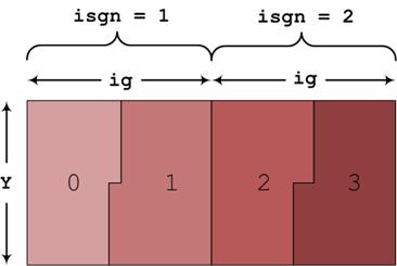
Figure 1: Example of how the data will be distributed
between 4 processes, when the allowed range for naky is divisible by two. The colour indicates
the process-id to which each piece of data is assigned.
Figure 1 shows the situation where the three
indices (naky,(2*ntgrid+1),isgn) can be evenly divided across four
processes, which is only possible if naky (Y) is even. If, on the other hand, naky were odd, the work would not divide evenly
over 4 processes, as indicated in Figure
2. This results in most processes being
allocated the same amount of data, but can very easily result in the situation,
especially for large problems and process counts, where one or more of the last
processes in the simulation will have little or no work assigned to them (i.e.
their allocated blocksize will be small or zero). While for large task counts
this will not result in a significant load imbalance in the computational work, it can dramatically increase the level of
communication that is required in the redistribution routines between xxf_lo and yxf_lo.
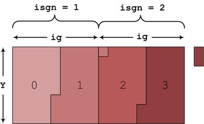
Figure 2: Example of a decomposition that does not
evenly split. In this example process 0 gets more than ½ of the first box, and
process 1 is then assigned some data points from the second box. When all the
data from the first two boxes are assigned, process 3 will still require data
from the next pair of boxes, as indicated by the small box to the right of the
main picture.
We now consider
the amount of data that must be passed between different processes during the
transformation between xxf_lo and yxf_lo. Figure 3
illustrates what happens when both indices split evenly across the processes,
clarifying that only a small amount of the data held by a process needs to be
transferred between neighbouring processes.
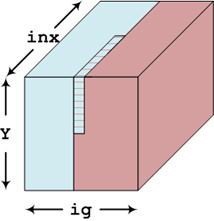
Figure 3:
Example of the data to be transferred between cores when transposing from xxf_lo to yxf_lo. For xxf_lo,
the lower ranking process holds the blue data and the shaded region. The higher
ranked process holds the red data. During the transformation the shaded region
needs to be transferred from the lower to the higher rank. There is a similar
region in the bottom rear of the cube, not visible in the figure, which needs
transferring from the higher ranking to the lower ranking process.
Figure 2 showed that,
if xxf_lo or yxf_lo data spaces do
not divide evenly across all processes, the equal blocksizes allocated to each
process will ensure all the data is allocated, but not that all processes will
be allocated data. The number of idle
processes can be calculated in the following equation:
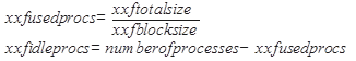
Similarly the idle
processes when using yxf_lo can be determined as follows:
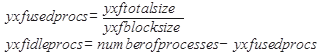
If the numbers yxf_idleprocs and xxf_idleprocs differ significantly, it can easily be
shown that large MPI messages will be required in the transforms between xxf_lo and yxf_lo. Figure 4
demonstrates clearly how the amount of data to be sent to a different process
increases linearly with increasing task number. If the difference between yxf_idleprocs and xxf_idleprocs is larger than 1, the highest ranking processes
(those of rank k and above in Figure 4) will have to transfer all
of their data to different processes. Where the difference is less than one,
all processes will keep some of their data.
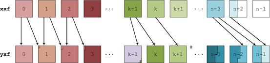
Figure 4: Example of the data redistributions required
when xxf_lo and yxf_lo have different numbers of idle
processors. The colours label the data regions that are stored by each
processor in xxf_lo.
If the decomposition used is undertaken
optimally it should be possible to ensure that the redistribution between g_lo and xxf_lo keeps X and Y as local as possible and thereby reduces or
eliminates completely the MPI communication in the xxf_lo to yxf_lo step.
Therefore, we have deliberately
created unbalanced decomposition functionality to optimise the data communications
in mapping from the xxf_lo and yxf_lo data layouts. The modified code replaces the current code
that calculates the block of xxf_lo
and yxf_lo owned by each
process, moving from a uniform blocksize to two different blocksizes for
process counts where the data spaces that preserve locality in x or y do not
exactly divide by the number of processes used.
The new, unbalanced, decomposition uses the process count to
calculate which indices can be completely split across the processes. This is
done by iterating through the indices in the order of the layout (so for the xxf_lo data distribution and the “xyles” layout this order would be s,e,l,isgn,ig,Y) dividing the number
of processes by each index until a value of less than one is reached. At this
point the remaining number of processes is used, along with the index to be
divided, to configure an optimally unbalanced decomposition, by deciding on how
to split the remaining indices across the cores that are available. If this
index dimension is less than the number of cores available, then the index
dimension is multiplied by the following index dimension until a satisfactory
decomposition becomes possible.
A worked example of the new decomposition algorithm is
provided in Appendix C.
This new functionality was benchmarked using two layouts (xyles at 2048 processes and yxles at 1536 processes), with the
results shown in the following table.
For the yxles layout the
computational imbalance created by the new code (the difference between the
small and large blocks) is approximately 5% and for xyles it is approximately 7%. This means that there is a 5% or 7%
difference in the amount of computational work that is performed in the
non-linear calculations between processes with the small and large blocks.
|
Number of Cores:
|
“yxles”
1536
|
“yxles”
1536 unbalanced
|
“xyles”
2048
|
“xyles”
2048 unbalanced
|
|
c_redist_22
|
Local Copy
|
13.89
|
43.13
|
30.20
|
32.59
|
|
|
Remote Copy
|
165.61
|
8.82
|
27.70
|
12.53
|
|
c_redist_22_inv
|
Local Copy
|
3.61
|
16.44
|
8.86
|
8.76
|
|
|
Remote Copy
|
48.19
|
2.43
|
4.78
|
2.99
|
|
c_redist_32
|
Local Copy
|
16.82
|
20.86
|
10.65
|
10.64
|
|
|
Remote Copy
|
217.45
|
196.81
|
110.66
|
116.11
|
|
c_redist_32_inv
|
Local Copy
|
2.77
|
3.48
|
1.97
|
1.79
|
|
|
Remote Copy
|
46.51
|
33.18
|
25.69
|
25.36
|
|
Total Calculation Time
|
2390.40
|
2074.20
|
1867.80
|
1862.40
|
Table 6:
Performance comparison of the code with and without the new unbalanced
decomposition functionality (using 10000 iterations)
We can see from
the results that the unbalanced decomposition can significantly improve the
performance obtained from the code.
Concentrating on the “yxles”
1536 results it is evident that moving from the original to the unbalanced code
the cost of the remote copy functionality for the c_redist_22 subroutines has been significantly reduced
(in fact almost removed altogether).
This is also mirrored in the corresponding inverse routine, and there
are also reasonable reductions in remote copy time for the c_redist_32 routine and its
inverse. This is balanced with an
increase in the local copy cost when using the unbalanced optimisation,
indicating that the unbalanced distribution has indeed ensured that the x and y
data has stayed local to processes wherever possible. Overall
the unbalanced optimisation saves around 15% of the runtime of GS2 for the yxles
layout on 1536 cores.
However, if we
look at the 2048 results (where the xyles layout
is used) the unbalanced optimisation makes little difference to the overall
runtime. The optimisation still
significantly reduces the runtime of the remote copy functionality in c_redist_22; however that
functionality is much less costly for this layout and process count. If we compare the “yxles” 1536 and “xyles”
2048 results the remote copy for c_redist_22
cost around 166 second in the 1536 case compared to around 28 seconds for the
2048 case. Therefore, the unbalanced
optimisation still does what we would expect for 2048 process using the xyles layout (i.e. significantly
reduces the cost of the c_redist_22
communications) but this layout and process count has little communication in
this routine in the first place so this optimisation does not have a
significant impact on the overall runtime of the simulation.
To understand
why there is this performance difference between the xyles and yxles
layouts on these process counts we need to examine the differences between the
two layouts. Both layouts have the same blocksizes
for the xxf_lo and yxf_lo data distributions (for a given
number of processes).
For “yxles” 1536 processes the original
code produces a xxf_lo blocksize
of 661⅓ which means that the y
index is split unevenly between groups of 2 or 3 processes (661⅓ ¸ ig
= 21⅓ which means that the first process has all the y indexes associated
with the first 21⅓ ig then
the second process has the y
indexes associate with the next 9⅔ ig
and then the following 11⅔ ig,
and so on, iterating through isgn,l,e,s). The actual blocksize used in GS2 must be an
integer (it isn’t possible to assign a fraction of a data entry to a process)
so for the data decomposition to work 661⅓ is rounded up to 662 and 662
elements are assigned to each process.
However, as this is a larger blocksize than the one actually needed in
the data decomposition then not all processes will be allocated data. The last process will have no data in the xxf_lo data distribution, and the
second to last process will only have a partial block of data. These two factors together mean that for “yxles” on 1536 processes there is a
large amount of data transfer required (as illustrated in Figure 4).
However, for
2048 processes the blocksize of 496 maps exactly to 2048 processes so all
processes have the same amount of data, and furthermore the y index is split evenly across pairs
of processes so the amount of data that has to be communicated is much smaller and
only needs to be transferred between pairs of processes. This leads to “xyles”
2048 processes having a much lower communication requirement for the
redistribution functionality than “yxles”
1536 processes. Indeed, at 2048
processes with the xyles layout
there is no need for the unbalanced optimisation as the decomposition is
already adequate, although the unbalanced decomposition functionality does not
damage the performance either.
The unbalanced
decomposition functionality also has the benefit of extending the range of optimal
process counts for a given GS2 simulation.
As previously discussed users generally select process counts for GS2
from the output of the ingen
program. This considers the factors of
each of the layout variables separately, in the order specified by the chosen
layout, and uses those to construct a list of process counts that match those
factors. The unbalanced decomposition
means that the list of suitable process counts can be much wider, including the
factors of a combination of the layout variables. Not only does this provide users with a wider
range of process counts to use, which can enable more efficient use of
different HPC resources (there is more scope to matching to the available
resource configuration i.e. number of cores per node, number of available
nodes, etc…), but also can reduce the runtime of the simulation by enabling the
selection of a more efficient layout and process count. An example of this is shown in Table 7 where
the performance of GS2 is shown with and without the unbalanced functionality
for the yxles layout. We can see good
performance improvements from using the unbalanced decomposition, however the
table also demonstrates that further optimisations can be achieved from using
from the yxles layout to the xyles layout when using the unbalanced
decomposition, even though 1536 processes was not an optimal process count for
the xyles layout with the original GS2.
|
Process Count
|
yxles, original decomposition
|
yxles, unbalanced decomposition
|
xyles, unbalanced decomposition
|
|
1536
|
7.07
|
6.12
|
5.94
|
Table 7: Performance improvement from
using the unbalanced decomposition and enabling different process counts for a
given layout.
We have undertaken a number of different optimisations on
the GS2 simulation code to improve the parallel performance and both allow the
code to scale more efficiently to larger numbers of cores and to complete
simulations quicker and therefore use less computational resources (HECToR AUs)
for any given scientific simulation.
Our primary focus was to improve the performance of the
local data copies associated with the data transform between the linear and
non-linear calculations in GS2. We
achieved this by replacing costly indirect addressing functionality by direct
access mechanisms reducing the cost of the routines performing the local data
copies by around 40-50%. This
optimisation has the most significant impact on performance at lower process
counts, as at larger core counts there is less data on each processor to be
kept local in the transformation, and therefore the performance is more
influenced by remote copies.
Following this optimisation we focussed on the remote copy
functionality associated with the same data transform. However, our optimisation attempts were not
successful for this particular functionality.
Finally, we were motivated to investigate optimising the
data decompositions used for the non-linear calculations. We discovered that the current functionality
that creates the data decomposition can lead to significant performance degradation
through increasing the amount of data to be transferred between processes for
the transform by a very large amount. We
implemented a new unbalanced decomposition that allocated slightly different
amounts of data to each process, in order to alleviate large communication
costs observed at large processes.
Combining these optimisations (the local copy optimisation that optimises performance for local
process counts and the unbalanced optimisation that can optimise performance
for higher process counts) we have been able to reduce the overall runtime
of the code by up to 17% for a representative benchmark, as shown in the
following table (where the code was run for 10000 iterations).
|
Number of Cores:
|
512
|
1536
|
|
Original Code
|
4435.20
|
2385.60
|
|
Indirect Addressing and Unbalanced Optimisations
|
4150.40
|
2074.20
|
|
Overall Percentage Optimisation
|
7%
|
17%
|
Table 8:
Overall performance improvement of GS2 (using the “xyles” layout for 512 and “yxles”
for 1536)
At 512 cores the data “xyles”
decompositions xxf_lo and yxf_lo keep BOTH x and y local, so the
unbalanced optimisation cannot play any useful role, but the optimisation of
the indirect addressing is still beneficial providing a 7% performance
improvement. At 1536 cores for “yxles” both the unbalanced
optimisation and the indirect addressing optimisation are beneficial, giving a
total improvement of 17% in the overall runtime of the simulation, despite the
fact that the unbalanced decomposition has introduced around 5% load imbalance
into the simulation. In addition to this,
using the “xyles” layout at 2048
with all the new functionality we have created reduces the runtime by just
under 20%, a significant saving of computational resources when considering the
75 Million AUs that have been or will be used by GS2 users on HECToR.
Furthermore, it is likely that the unbalanced decomposition
approach will be applicable to other scientific simulation codes where both
real space and k-space data domains are used.
The redistribution functionality that we have optimised is
also used in other parts of GS2, particularly in the collision functionality
within the code. Whilst we have not
studied that during this project it is likely that the local copy optimisation
we undertook during this work will be applicable to the part of GS2 that deals
with the collision operator and therefore that further performance optimisation
could be achieved by removing indirect addressing from this part of GS2 as
well.
Furthermore, removing indirect addressing from the model collision
operator functionality should also enable the code to be refactored to remove
the majority of the data structures required for the indirect addressing
functionality, hence saving valuable memory.
The new
functionality developed in this dCSE project has been undertaken using a branch
in the main GS2 SVN repository. All the
new code is available to the GS2 developers and they are currently working to integrate
this branch with the main GS2 trunk to ensure these developments can be
exploited by all GS2 users, including sister-codes AstroGK and Trinity (which
runs GS2 in parallel in multi-scale plasma simulations). We have also produced some separate
documentation on the GS2 layouts and how to use the new GS2 functionality;
including extending the ingen
tool that is used in conjunction with GS2 to ensure that GS2 is used in an
optimal manner.
This work
was supported by Colin Roach at CCFE and Joachim Hein at EPCC, The University
of Edinburgh.
This project was
funded under the HECToR Distributed Computational Science and Engineering (CSE)
Service operated by NAG Ltd. HECToR – A Research Councils UK High End Computing
Service - is the UK's national supercomputing service, managed by EPSRC on
behalf of the participating Research Councils. Its mission is to support
capability science and engineering in UK academia. The HECToR supercomputers
are managed by UoE HPCx Ltd and the CSE Support Service is provided by NAG Ltd.
http://www.hector.ac.uk
Appendix A – Input datafile
&theta_grid_knobs
equilibrium_option='eik'
/
&theta_grid_parameters
rhoc = 0.4
ntheta = 30
nperiod= 1
/
¶meters
beta = 0.04948
zeff = 1.0
TiTe = 1.0
/
&collisions_knobs
collision_model
= 'none'
!collision_model='lorentz'
/
&theta_grid_eik_knobs
itor = 1
iflux = 1
irho = 3
ppl_eq = .false.
gen_eq = .false.
vmom_eq = .false.
efit_eq = .true.
gs2d_eq = .true.
local_eq = .false.
eqfile = 'equilibrium.dat'
equal_arc = .false.
bishop = 1
s_hat_input = 0.29
beta_prime_input = -0.5
delrho = 1.e-3
isym = 0
writelots = .false.
/
&fields_knobs
field_option='implicit'
/
&gs2_diagnostics_knobs
write_ascii = .false.
print_flux_line
= .true.
write_flux_line
= .true.
write_nl_flux = .true.
write_omega = .false.
write_omavg = .false.
write_phi =.true.
write_final_moments
= .false.
write_final_fields=.false.
print_line=.false.
write_line=.false.
write_qheat=.true.
write_pflux=.false.
write_vflux=.false.
write_qmheat=.false.
write_pmflux=.false.
write_vmflux=.false.
print_old_units=.false.
save_for_restart=.false.
nsave= 500
nwrite= 100
navg= 200
omegatol= 1.0e-5
omegatinst = 500.0
/
&le_grids_knobs
ngauss = 8
negrid = 8
Ecut = 6.0
advanced_egrid = .true.
/
&dist_fn_knobs
boundary_option=
"linked"
gridfac= 1.0
/
&init_g_knobs
!restart_file= "nc/input.nc"
ginit_option= "noise"
phiinit= 1.e-6
chop_side = .false.
/
&kt_grids_knobs
grid_option='box'
norm_option='t_over_m'
/
&kt_grids_box_parameters
y0 = 10
ny = 96
nx = 96
jtwist = 2
/
&knobs
fphi= 1.0
fapar= 0.0
faperp= 0.0
delt= 1.0e-4
nstep= 500
wstar_units = .false.
/
&species_knobs
nspec= 2
/
&species_parameters_1
type = 'ion'
z = 1.0
mass = 1.0
dens = 1.0
temp = 1.0
tprim = 2.04
fprim = 0.0
vnewk = 0.0
uprim = 0.0
/
&dist_fn_species_knobs_1
fexpr = 0.45
bakdif = 0.05
/
&species_parameters_2
type = 'electron'
z = -1.0
mass = 0.01
dens = 1.0
temp = 1.0
tprim = 2.04
fprim = 0.0
vnewk = 0.0
uprim = 0.0
/
&dist_fn_species_knobs_2
fexpr= 0.45
bakdif= 0.05
/
&theta_grid_file_knobs
gridout_file='grid.out'
/
&theta_grid_gridgen_knobs
npadd = 0
alknob = 0.0
epsknob = 1.e-5
extrknob = 0.0
tension = 1.0
thetamax = 0.0
deltaw = 0.0
widthw = 1.0
/
&source_knobs
/
&nonlinear_terms_knobs
nonlinear_mode='on'
cfl =
0.5
/
&additional_linear_terms_knobs
/
&reinit_knobs
delt_adj = 2.0
delt_minimum = 1.e-8
/
&theta_grid_salpha_knobs
/
&hyper_knobs
/
&layouts_knobs
layout = 'xyles'
local_field_solve
= .false.
/
Appendix B – Further optimised c_redist_32 code
t1upper = ubound(to_here,1)
f3upper = ubound(from_here,3)
tempnaky = naky
innermaxmultiplier = xxf_lo%ulim_proc+1
select case (layout)
case ('yxels')
f3maxmultiple = xxf_lo%naky*xxf_lo%ntheta0
f3incr = xxf_lo%naky
case ('yxles')
f3maxmultiple = xxf_lo%naky*xxf_lo%ntheta0
f3incr = xxf_lo%naky
case ('lexys')
f3maxmultiple = xxf_lo%nlambda*xxf_lo%negrid*xxf_lo%ntheta0
f3incr = xxf_lo%nlambda*xxf_lo%negrid
case ('lxyes')
f3maxmultiple = xxf_lo%nlambda*xxf_lo%ntheta0
f3incr = xxf_lo%nlambda
case ('lyxes')
f3maxmultiple = xxf_lo%nlambda*xxf_lo%naky*xxf_lo%ntheta0
f3incr = xxf_lo%nlambda*xxf_lo%naky
case('xyles')
f3maxmultiple = xxf_lo%ntheta0
f3incr = 1
end select
i = 1
iglomax = ((iproc+1)*g_lo%blocksize)
t1test = ((xxf_lo%ntheta0+1)/2)+1
do while(i .le. r%from(iproc)%nn)
f1 = r%from(iproc)%k(i)
f2 = r%from(iproc)%l(i)
f3 = r%from(iproc)%m(i)
t1 = r%to(iproc)%k(i)
t2 = r%to(iproc)%l(i)
outerf3limit = f3 + f3incr
do while(f3 .lt. outerf3limit)
iincrem = i
innermaxrealvalue = (innermaxmultiplier-t2)/tempnaky
innermax = ceiling(innermaxrealvalue)-1
if(f2 .eq. 2 .and. (f1+innermax) .gt. ntgrid) then
innermax = i + (ntgrid - f1)
else if((f2 .eq. 1 .and. innermax .gt. (((2*ntgrid)+1)+(ntgrid-f1)))) then
innermax = i + ((2*ntgrid)+1) + (ntgrid - f1)
else
innermax = i + innermax
end if
do while(i .le. innermax)
f1 = r%from(iproc)%k(i)
f2 = r%from(iproc)%l(i)
f3 = r%from(iproc)%m(i)
t1 = r%to(iproc)%k(i)
t2 = r%to(iproc)%l(i)
startf3 = f3
f3max = ((f3/f3maxmultiple)+1)*f3maxmultiple
f3max = min(f3max,iglomax)
do while (f3 .lt. f3max)
to_here(t1,t2) = from_here(f1,f2,f3)
f3 = f3 + f3incr
t1 = t1 + 1
if(t1 .eq. t1test) then
t1 = t1 - xxf_lo%ntheta0 + xxf_lo%nx
end if
iincrem = iincrem + 1
end do
i = i + 1
end do
if(i .lt. r%from(iproc)%nn .and. iincrem .lt. r%from(iproc)%nn) then
f1 = r%from(iproc)%k(i)
f2 = r%from(iproc)%l(i)
t2 = r%to(iproc)%l(i)
f3 = startf3 + 1
else
f3 = outerf3limit
end if
end do
i = iincrem
end do
Appendix C – Worked example of the unbalanced decomposition algorithm
To illustrate the unbalanced decomposition algorithm with an
example, for the benchmarking in this document we have generally been using the
following parameters:
·
y
= 32
·
ig
= 31
·
isgn
= 2
·
l
= 32
·
e
= 8
·
s
= 2
For the xxf_lo data
distribution, using 1536 processes, the unbalanced code does the following:
·
1536 ¸ s = 768
·
768 ¸ e = 96
·
96 ¸ l = 3
·
3 ¸ isgn
= 1.5, this is not whole so carry isgn forward
·
3 ¸ isgn
* ig < 1, this is the point to create the
unbalanced blocks
The unbalanced block sizes are then created using the
remaining number of processes (3) and the index(s) to be split (isgn
* ig = 62),
as follows:
·
62 ¸ 3 =
20⅔
·
This gives two sizes, 20 and 21. We have 3 blocks required, one of 20 and two
of 21 provide the 62 required
·
20 and 21 are then used to calculate the xxf_lo blocksize by multiplying the remaining
indexes (those not split) by the two blocks calculates
·
Blocksize 1 = 20 * y = 640
·
Blocksize 2 = 21 * y = 672
·
The original blocksize for this example is 662
·
The new blocksize is 640 for ⅓ of the
processes and 672 for ⅔ of the processes
·
Original data domain was y * ig * isgn * l
* e * s = 1015808
·
1015808 / 1536 = 661⅓ = original blocksize
= 662
·
640 * (⅓ * 1536) + 672 * (⅔ * 1536)
= 1015808
·
The new blocksizes exactly decompose the data
domain over the number of processes used.
Appendix D – Optimised Local Copies, Optimal Core Counts and Domain Decompositions in Nonlinear GS2 Simulations
The updated GS2
code has been altered to allow users to select whether to use unbalanced
decompositions or not. With this new
functionality the user should select a processor count that is optimal for the
linear calculations and utilise the unbalanced optimisation code within GS2 by
setting the following variables in the parameters input file (in the section &layouts_knobs):
unbalanced_yxf = .true.
max_unbalanced_yxf = 0.15
unbalanced_xxf = .true.
max_unbalanced_xxf = 0.15
The value 0.15
using for the two max_unbalanced_*
parameters sets the maximum amount of unbalance allowed in the decompositions;
0.15 sets this as a maximum of 15% but this can be chosen by the user (a
default of zero is set if nothing is chosen by the user which forces the
unbalanced code not to be used, and the maximum is 1.0). This enables users to cap the amount of
computational imbalance that is introduced into the code to address these performance
issues to ensure that the performance improvements achieved through the
unbalanced functionality and not negated by the added computational imbalance.
The ingen utility that accompanies GS2 has
also been updated to ensure that those core counts that it suggests (those
optimal for the linear calculations) that are not optimal for the nonlinear
calculations are annotated with suggestions for the flags to set in the input
file to activate the required unbalanced functionality.
The new
optimised local copy functionality can be enabled or disabled using the
following variable in the parameters input file (in the section &layouts_knobs):
opt_local_copy = .true.
If this
parameter is set to .false. or omitted from the parameter input file
then the optimised local copy functionality is not used. If it is set to .true. then the
optimised local copy will be used.