Forecasting Faster: Configuring and Optimising the Weather Research & Forecast Model for Maximum Performance
Dr Andy Porter, Advanced Research Computing Group, STFC Daresbury Laboratory
Understanding and predicting the behaviour of the Earth's atmosphere and weather systems is a very complex problem and has historically always exercised the leading High Performance Computing resources available at any one time. The significant usage of HECToR for atmosphere-related simulation work continues this trend and the Weather Research & Forecast (WRF) Model accounts for a large part of this. In this HECToR dCSE project [1], we have investigated various ways in which the performance of WRF on Phase 2a of HECToR may be improved.
The WRF model was developed as a collaborative project by several organisations in the United States. It is a regional- to global-scale model intended for both research applications and operational weather-forecast systems. WRF is used in the US as the National Oceanic and Atmospheric Administration's primary forecast model for forecasts of 1 - 3 days ahead, and is used by weather agencies all over the world (including weather agencies in Indo-China and Asia). As of June 2008 there were in excess of 6000 registered WRF users.
The WRF system incorporates two different dynamics solvers; the Advanced Research WRF (ARW) solver (developed by the Mesoscale and Microscale Meteorology Division of NCAR) and the Non-hydrostatic Mesoscale Model solver (developed by the National Centers for Environmental Prediction, US). In this work we deal only with the ARW version of the WRF modeling system.
The ARW solves the fully-compressible, non-hydrostatic Euler equations using a finite-difference scheme on an Arakawa C-grid staggering in the horizontal plane and a terrain-following, dry hydrostatic pressure vertical coordinate. There are 2nd- to 6th-order advection options for spatial discretization in both horizontal and vertical directions. Integration in time is performed using a time-split method with a 2nd- or 3rd-order Runge-Kutta scheme with a smaller time step for acoustic- and gravity-wave modes. The model supports periodic, open, symmetric and specified lateral boundary conditions and is capable of whole-globe simulations using polar Fourier filtering and periodic east-west boundary conditions.
The WRF model has, from the outset, been designed and written to perform well on massively-parallel computers. It is written in Fortran90 and can be built in serial, parallel (distributed or shared memory) and mixed-mode (distributed and shared memory) forms, simply by choosing the appropriate option during the configuration process.
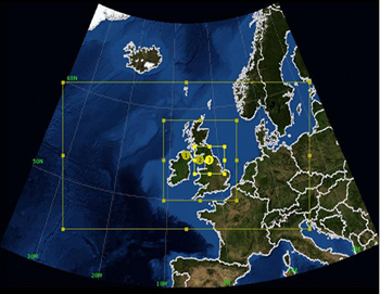
Figure 1. The three domains for the Great North Run benchmarking
configuration
The majority of the WRF runs done in this project used the "Great North Run" (GNR) configuration, chosen to be representative of the WRF-related work done by the UK community on HECToR. This configuration is shown in figure 1 and consists of three, nested domains with two-way feedback between them. It is designed to provide a `Weather Forecast' for the north of England which is thus covered by a small domain of high-resolution (1 Km). This configuration is used by the National Centre for Atmospheric Science, UK, as both a teaching tool and for use with scientific field campaigns being carried out in the UK.
When measuring the performance of WRF we have used the mean time taken to integrate the whole model forwards in time by one time step. Typically, the mean value was calculated from three separate runs of 10 minutes of model time. This quantity explicitly excludes any time spent doing Input/Output (I/O).
Choice of compiler and build mode
WRF is supplied with its own, interactive "configure" script which seeks to identify the platform and offer appropriate options. On HECToR where the Portland Group (PGI), Pathscale (PS), Gnu and Cray compiler suites are installed, this results in approximately 20 different ways of building WRF! However, the relatively-young Cray compiler was unable to build WRF and therefore was not an option for this project.
We found that the PGI compiler produced the best-performing WRF executable when it was built in distributed-memory (MPI) only mode. (In this mode, the model domain is split into "patches" and each computational core is assigned one of them to work on.) The PS compiler came a close second while the executable produced by the Gnu compiler was typically 10-20% slower on core counts up to 1024.
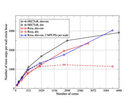
Figure 2. The performance of WRF running the GNR configuration on the
HECToR and Rosa machines. The MPI-only binary was built with the PGI
compiler and the mixed-mode binary with the PS compiler. Compute
nodes were fully occupied for these jobs.
The most significant improvement in performance was obtained when WRF was built in mixed-mode. In this case, typically just one MPI process is run on each compute node of the machine. The patch of the model domain associated with this process is then further decomposed into `tiles' which are shared out amongst the OpenMP threads that are run on the cores of the compute node. For WRF in this mode, the PS compiler was found to be best. Figure 2 compares the performance of WRF built in mixed mode with that built in distributed-memory mode on both HECToR Phase IIa and on Rosa; a Cray XT5 at CSCS in Switzerland. Below 512 cores, the mixed-mode binary is slightly slower than the pure MPI version. However, on larger core counts where communication overheads increase, the mixed-mode binary is significantly faster, presumably due to its reduction of the MPI communication between cores. Even better performance is obtained on the Cray XT5 when the job uses one MPI process per socket (multi-core chip) and OpenMP threads across the cores within the socket.
These results indicate that the mixed-mode version of WRF is essential to maintaining performance levels on the increasingly fat nodes of current massively-parallel machines. This is borne out by its performance on the Cray XT5 which has 12 cores per node compared to HECToR Phase IIa's four.
Tiling to improve cache usage
The further decomposition of domain patches into tiles used in the mixed-mode implementation is not tied to the number of OpenMP threads being used or in fact to the use of OpenMP at all. This means that the user is free to alter the number of tiles/patch at run time in order to tune the size of the arrays within the computation to make more efficient use of the cache architecture of the AMD processor.
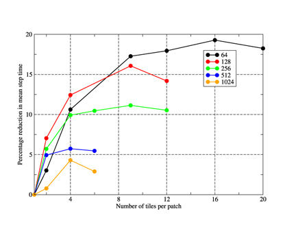
Figure 3. The percentage reduction in the mean wall-clock time taken to
step the model as a function of the number of tiles used per
patch. Results are shown for a variety of PE counts for the GNR
configuration. Lines are guides to the eye
Figure 3 shows the effect on the performance of WRF (built in MPI mode) when the number of tiles per patch is increased. As one would expect, the use of tiling has the greatest effect on the lower PE counts when the patches and thus array extents are at their largest and therefore do not fit into cache. So we see that using 16 tiles/patch on a 64-PE job achieves a speed-up of almost 20% whilst the best achieved for the 1024-PE job is approximately 5% with just four tiles/patch.
IO techniques
Codes like WRF must periodically write large quantities of data to disk while they run and this can often be a significant performance bottleneck.
The default approach to outputting a distributed array in WRF is to gather all of the data onto the master PE using a call to MPI_Gatherv, reconstruct the array and then write it to disk using the standard, serial netCDF library. Finally, the number of bytes written to disk is broadcast back to all PEs which means that all PEs block until the master has completed the write. The time taken to do all of this for each domain is written to standard output and it is this figure that has been used in this study. Since it includes the time taken by the call to MPI_Gatherv, it is not strictly the time taken to write the data to disk but, more importantly, it is the amount of wall-clock time "lost" due to doing the output.
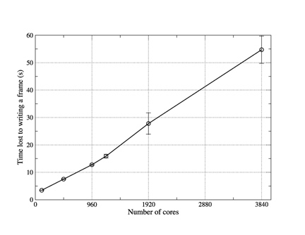
Figure 4. The time "lost" to writing a single frame of history data using
pNetCDF as the number of cores used in the WRF job is increased. Each data
point represents the mean value obtained from three separate runs on
Rosa and error bars show the associated standard error. Lines are
guides to the eye.
WRF also comes with an I/O layer implemented with pNetCDF - an extension of the netCDF library that supports parallel I/O. Unfortunately WRF is written such that when it is built to use this layer, every PE writes its part of the data to disk. On large PE counts, each of these writes is then for a relatively small amount of data and the large number of writers accessing a single file can cause contention. This is illustrated by the results (obtained on the Cray XT5) shown in figure 4 where the time lost to writing out a single frame of history can be seen to increase almost linearly with the number of cores being used. Although it might be possible to improve this performance by tuning the underlying parallel filestystem, it is clear that this method will not scale to very high PE counts.
It appears therefore that, as implemented, the pNetCDF layer in WRF is best suited to the case where the amount of memory available to any individual PE is insufficient to permit the gathering of data to a single writer.
As described above, in the default I/O layer all of the PEs must wait for the master PE to finish writing the history data to disk before proceeding with the computation. A useful optimisation therefore is to set aside one or more PEs for dealing exclusively with I/O. Once the "compute" PEs have transmitted their data to these "IO servers" they are free to continue with the calculation without waiting for the data to actually be written to disk. WRF contains such functionality with the user able to select how many PEs to dedicate to I/O at run time through the "namelist_quilt" section of the input file. The IO servers themselves reconstruct the field to be to be written on the master IO server which then writes it to disk using one of the serial WRF I/O layers (netCDF in this case).
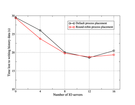
Figure 5. The mean time "lost" by each of the compute nodes when
writing a single history frame. WRF was run with 1024 compute PEs
plus the specified number of IO servers.
We tested the performance of this functionality on HECToR for a job consisting of 1024 compute PEs and the results are shown in figure 5. Essentially, use of the IO servers reduces the time "lost" by the compute PEs in writing a single frame of history from 30 to 19 seconds. The optimum number of IO servers in this particular case is 12 so that there are approximately 85 compute PEs per server.
In terms of scalability, this asynchronous method is the best approach to I/O currently implemented in WRF. However, it retains the critical limitation that the whole model domain must fit into the memory of a single PE. Work has subsequently been done to lift this restriction by extending the IO servers to do parallel I/O and this feature is scheduled to be made available in the spring 2011 release of WRF.
References
[1] A. R. Porter, M. Ashworth, A. Gadian, R. Burton, P. Connolly and M. Bane, WRF code Optimisation for Meso-scale Process Studies (WOMPS) dCSE Project ReportAcknowledgements
Invaluable problem-solving assistance was provided by one of the WRF code authors, John Michalakes of the National Renewable Energy Laboratory, US.
This work was funded under a HECToR Distributed Computational Science and Engineering (dCSE) grant from NAG Ltd.