
1Edinburgh Parallel Computing Centre, The University of Edinburgh, United Kingdom
2School of Mathematical Sciences, University College Dublin, Ireland
3Institute for Materials and Processes, The University of Edinburgh, United Kingdom
4Département Mécanique, Université de Lyon 1 and Laboratoire de la Mécanique des Fluides & d’Acoustique (LMFA), CNRS, Ecole Centrale Lyon, Ecully, France
19th June 2013
Abstract
The performance and sustainability of a fully parallelised 3-dimensional two-phase Navier-Stokes flow solver called TPLS (Two Phase Level Set) has been improved. The most expensive area of computation in the TPLS code is the pressure calculation which was originally implemented using successive over-relaxation. This has been replaced by calls to the PETSc library which allows various preconditioners and Krylov solvers to be used. In addition some optimisation of MPI communications has been carried out. An improvement in performance of up to 54% in the pressure solver has been achieved. This has enabled two-phase flow simulations at ultra-high resolution for a variety of engineering applications. For example the TPLS solver is being used to understand two-phase counter-current flows in carbon capture processes. There are a number of related projects in which the code will be used, including a current EPSRC grant which is concerned with cooling microelectronic devices via evaporating coolants in microchannels. The work reported here contributes directly to the increased accuracy of simulations used to inform the engineering design of these channels. The optimised code has now been released to the community under an open-source BSD license.
This is the final report for a dCSE project that ran from 1st July 2012 to 30th April 2013.
Dr. Lennon Ó Náraigh and Dr. Prashant Valluri have developed a two-phase Navier-Stokes flow solver called TPLS. This uses the level-set method (see [1] for a general desription) to calculate the dynamic evolution of a 3D interface in addition to the complete flow field information such as velocity vector and pressure fields. It accurately describes two-phase laminar flow in channel geometries. The code uses a hybrid MPI/OpenMP parallelisation strategy and scales well up to 1,000 CPU cores when employed to solve problems involving up to 8 million grid points. The code can be used to gain practical understanding of problems of interest to the oil and gas industry as well as for carbon capture and storage applications, among others. In addition it can be used to obtain theoretical insight into two-phase interfacial instability. However there is an need to obtain results for larger grids, to obtain better accuracy, and model wider and longer channels. There were doubts as to how well the code would scale beyond 1,000 cores and consequent worries about the length of execution times. This document reports on our work to improve the scalability of the code and to optimise the pressure solver which implements the most expensive part of the computation.
Ó Náraigh and Valluri have also developed a 3D, two-phase, Navier-Stokes solver with a diffuse-interface method (DIM) for interface capturing (see [2] for a general description). This is a purely OpenOMP code and so cannot employ large numbers of cores. We planned to introduce MPI parallelisation to this code using methods similar to those used in the TPLS code, although this was not achieved within the duration of the project.
The primary aim of this project was to enable TPLS and DIM to utilise HECToR for the simulation of flows on grids with at least 24 million points. The ability to model high-resolution geometries will then help improve our understanding of complex interfacial phenomena in two-phase flows.
The project had three objectives:
Two changes were made to the work plan:
Reinterpreting the deliverables with these changes in mind one can say that
In all of the work reported here the Fortran compiler used was gfortan 4.7.2, with the -O3 flag. The version of PETSc used was 3.3. All timings are given in seconds.
This dCSE project was carried out on HECToR, the UK National Supercomputing service, and its associated Test and Development System. HECToR was in its Phase 3 configuration. Full details of the system are available on its website http://www.hector.ac.uk.
In the initial version of the code, the pressure is calculated using a combination of Jacobi’s method and successive over-relaxation (S.O.R.) iterative solvers. A single iteration consists of a red-black S.O.R. scheme with a single Jacobi step between the red and black updates. Whilst some information on residuals is generated it is not used to control the iterative process, instead fixed numbers of iterations are used. For each of the first 100 hundred time steps 1000 iterations are performed by the pressure solver. After that 300 iterations are performed per time step.
One of the boundary conditions employed was found not to be suitable for use with a Krylov solver. The code was re-written slightly by Ó Náraigh so that a standard von Neumann boundary condition was used instead, with no measurable impact on the output of the code.
In this subsection timings are given for simulations of a 512×144×152 domain using 1,024 cores. The first row shows how the cores are employed: the first number is the number of MPI processes in the x-direction, the second is the number of MPI processes in the y-direction, whilst the third number is the number of OpenMP threads per MPI process. There is always a single MPI process in the z-direction as TPLS employs a 2D data decomposition.
Figures are given for both the original code and the code with modified boundary conditions.
| 16×8 - 8 | 32×8 - 4 | 32×16 - 2 | 64x16 - 1 | |
| Original | 22095 | 20523 | 17921 | 19906 |
| New BC’s | 21736 | 20722 | 17292 | 19507 |
Table 1: Overall time for 25,000 time steps excluding initialisation
| 16×8 - 8 | 32×8 - 4 | 32×16 - 2 | 64x16 - 1 | |
| Original | 12955 | 11480 | 8205 | 7169 |
| New BC’s | 12984 | 11488 | 8222 | 7095 |
Table 2: Time for 25,000 time steps excluding output and initialisation
As was expected the change of boundary conditions does not affect the execution speed of the code.
What was unexpected is that better performance is achieved when using only one OpenMP thread. This contradicts what was found in a previous study, prior to the dCSE project. The choice of using several threads was optimal on HECToR Phase 2b, but is no longer the case on Phase 3, where the ’Gemini’ interconnect can comfortably sustain traffic from a larger number of MPI processes per node.
Note that a lot of time (over 50% in some cases) is spent performing output. In the subsequent analysis this must be taken into account in order to reveal the behaviour of other parts of the code.
In what follows, unless there is a statement to the contrary, exactly one OpenMP thread is used per MPI process. Also the term ’reference code’ means the TPLS code with modified boundary conditions.
In this subsection the scaling of the reference code is discussed.
Strong scaling refers to how the performance of the code varies with the number of cores for a fixed problem size (domain). Weak scaling refers to how the performance of the code varies with the number of cores for a problem size proportional to the number of cores (so that the size of the sub-domain associated with each core remains constant). For strong scaling the efficiency of one run compared to another run is defined as
where the subscripts refer to the run (1 indicating that the smaller number of cores were used and 2 the larger), t denotes a timing and cores is the number of cores used in the run. For weak scaling the efficiency of one run compared to another run is defined as

| Cores | Total Time | Output | Total Comp. | Pressure | Other |
| 1024 | 19507 | 12412 | 7095 | 4084 | 3011 |
| 2048 | 17734 | 12410 | 5322 | 3243 | 2079 |
| Efficiency | 0.5 | 0.5 | 0.7 | 0.6 | 0.7 |
Table 3: Strong scaling for a 512×144×152 domain
| Cores | Total Time | Output | Total Comp. | Pressure | Other |
| 1024 | 19507 | 12412 | 7095 | 4084 | 3011 |
| 2048 | 32253 | 25095 | 7158 | 4132 | 3026 |
| Efficiency | 0.6 | 0.5 | 1 | 1 | 1 |
Table 4: Weak Scaling for 512×144×152 versus 1024×144×152
The output does not scale at all. This is because the data is gathered onto the master process and written out from there i.e. the output is serialised.
For the computational part of the code (the non-output part) weak scaling is excellent. Strong scaling is less good (although still reasonable) due to the relative increase in cost of halo swapping compared to computation.
In this subsection the performance of an optimised version of the reference code is described. Some redundant code has been removed (such as a number of MPI barriers and some OpenMP collective operations) and some tuning of the OpenMP directives has been attempted. Also non-blocking point-to-point communications have been introduced to allow multiple communications to be overlapped, reducing latency. Speed-up is defined as

where the subscript 1 refers to the reference code whilst 2 refers to the optimised code and t denotes a timing.
Only the introduction of non-blocking point-to-point communications produced a measurable speeding up of the code.
| 16×8 - 8 | 32×8 - 4 | 32×16 - 2 | 64x16 - 1 | |
| Reference | 21736 | 20722 | 17292 | 19507 |
| Optimised | 21516 | 20200 | 17065 | 18780 |
| Speed-Up | 1% | 2.6% | 1.3% | 3.9% |
Table 5: Timings for the codes including output.
| 16×8 - 8 | 32×8 - 4 | 32×16 - 2 | 64x16 - 1 | |
| Reference | 12984 | 11488 | 8222 | 7095 |
| Optimised | 12390 | 11041 | 7538 | 6333 |
| Speed-Up | 4.8% | 4% | 9.1% | 12% |
Table 6: Timings for the codes excluding output.
1,024 cores were used. Again there is no benefit in using OpenMP threads but using non-blocking sends and receives produces a measurable benefit. When output is excluded the target speed-up is slightly exceeded.
The pressure solver of the reference code was replaced by calls to routines in the PETSc library. As in the reference code only the x an y dimensions were parallelised. The PETSc library is written in C but it has a Fortran 90 interface which was used in this work. It took considerable time to learn how to use the PETSc library because of a lack of good documentation (particularly of the Fortran interface).
When initialising the Krylov solver, and when extracting data from it at each time step, the data had to be rearranged to conform to the arrangement of the data in the rest of the code. This was for two reasons:
The performance penalty associated with this rearrangement was small (although it could be removed entirely if the rest of the code was converted over to use PETSc).
Experimentation with the PETSc library demonstrated that stability was a problem in the initial stages of the simulation. The only satisfactory solver that we found was the Generalised Minimal Residual (GMRES) solver. The Conjugate Gradient solver did not converge at first but could be used after 4,000 time steps. However, even then, it displayed no performance improvement over GMRES. All of the results reported below for the PETSc version of the code were generated using GMRES with a Block Jacobi preconditioner.
The convergence criterion that was used in the runs was that the relative decrease in the preconditioned residual norm should be less than 0.0001. Using PETSc it is not possible to fix the number of iterations that the solver uses (as is the case in the reference code) but, as will be discussed later, one can limit the number used.
In this subsection the scaling of the PETSc version of the code is examined.
| Cores | Total Time | I/O | Total Comp. | Pressure | Other |
| 1024 | 18680 | 12497 | 6183 | 3432 | 2751 |
| 2048 | 16270 | 12560 | 3710 | 1784 | 1926 |
| Efficiency | 0.6 | 0.5 | 0.8 | 1 | 0.7 |
Table 7: Strong scaling 512×144×152
| Cores | Total Time | I/O | Total Comp. | Pressure | Other |
| 1024 | 18680 | 12497 | 6183 | 3432 | 2751 |
| 2048 | 34188 | 24842 | 9346 | 6597 | 2749 |
| Efficiency | 0.5 | 0.5 | 0.7 | 0.5 | 1 |
Table 8: Weak Scaling - 512×144×152 versus 1024×144×152
In these experiments the ’other’ (i.e. non-pressure) part of the computation (excluding output) was identical to that of the optimised code described above. By comparing Tables 7 and 8 to Tables 3 and 4 respectively we can see that the scaling of this part of the code is the same as that of the reference code. The improvement in performance produced by the optimisations is also evident.
The weak scaling performance of the PETSc version of the code is so poor because of the large number of iterations required to achieve convergence in the first 4,000 (approximately) time steps. In the case of the 512×144×152 domain the maximal number of iterations required for a time step was 1,770 (with about 14 needed for time steps towards the end of the run) whilst for the 1024×144×152 domain it was 4,697 (again with about 14 needed for time steps towards the end of the run). If only later time steps are considered the efficiency of the pressure calculation is 1 as will be shown below.
The larger domain has more than 22 million grid points. The largest domain that has been simulated had 27 million grid points. The dimensions of the latter domain did not suit the analysis reported here and it is not discussed further.
In this subsection the performance of the PETSc version of the code is compared to that of the reference code as the number of OpenMP processes is varied whilst employing a fixed number of cores (1,024). Inspection of residual norms in a few cases near the ends of the simulations suggested that the final accuracy of the reference and PETSc codes was similar.
| 16×8 - 8 | 32×8 - 4 | 32×16 - 2 | 64x16 - 1 | |
| Reference | 21736 | 20722 | 17292 | 19507 |
| PETSc | 25527 | 21512 | 19220 | 18680 |
| Speed-Up | -15% | -4% | -10% | 4% |
Table 9: Timings for the codes including output
| 16×8 - 8 | 32×8 - 4 | 32×16 - 2 | 64x16 - 1 | |
| Reference | 12984 | 11488 | 8222 | 7095 |
| PETSc | 16378 | 12417 | 7537 | 6183 |
| Speed-Up | -21% | -7% | 9% | 15% |
Table 10: Timings for the codes excluding output
Again one can see that there is no benefit form using OpenMP threads. This is not surprising for the PETSc code as the PETSc library does not use OpenMP at all.
Excluding output, the best speed-up achieved over 25,000 time steps is 15%.
Next the performance of the pressure solver excluding transient behaviour at the beginning of the run will be examined. Throughout three runs of 25,000 time steps the time taken by the pressure solver to complete blocks of 100 time steps was measured. The three runs were characterised by the following parameters:
These are the runs previously used to examine the scaling behaviour of the code.
Figure 1 shows the results. Rather than plotting the absolute time required for each block of 100 time steps the natural logarithm of the ratio of the time required by the block to the time required by the corresponding block of 100 time steps in the reference code is plotted. In more detail:
The peak for each run does not occur for block 1 because of the fact that 1,000 iterations used by the reference code in the first one hundred time steps after which the average time required for 300 iterations is used to perform the comparison.
As can be seen there is strong transient behaviour during the first 4,000 or so iterations. The speed-up of the pressure calculation in the PETSc code relative to the reference code for the last 20,000 time steps is given in Table 11 and is excellent. Strong and weak scaling of the PETSc code are examined in Tables 11 and 12 respectively. They too show excellent behaviour for the last 20,000 time steps. So the PETSc code easily outperforms the reference code if the initial period of the simulation is ignored (or can be improved, as we now show).
| 1024:512 | 2048:512 | 2048:1024 | |
| Reference | 3237 | 2570 | 3276 |
| PETSc | 1291 | 702 | 1303 |
| Speed-Up | 151% | 266% | 151% |
Table 11: Timings for the pressure calculation excluding the first 5000 time steps
| Cores | Pressure |
| 1024 | 1291 |
| 2048 | 702 |
| Efficiency | 0.9 |
Table 12: PETSc strong scaling 512×144×152 excluding the first 5000 time steps
| Cores | Pressure |
| 1024 | 1291 |
| 2048 | 1303 |
| Efficiency | 1 |
Table 13: PETSc weak Scaling - 512×144×152 versus 1024×144×152 excluding the first 5000 time steps
![]()
Figure 1 - Relative performance of the pressure calculation. The series are labelled x_dim:core_count
Note that after 50 blocks the plots for the runs employing 1,024 cores on a 512×144×152 domain and 2,048 cores on a 1024×144×152 domain coincide. This demonstrates perfect weak scaling for these grid sizes beyond the 50th block.
It is possible to restrict the number of iterations that PETSc performs. Given that the reference code produces acceptable results whilst using a fixed number of iterations we investigated if the PETSc code would do the same. If this were the case then the overall performance of the PETSc code would be improved. This has yet to be investigated thoroughly but preliminary results look promising. A simulation of a 512×144×152 domain on 1,024 cores has been performed with the number of iterations performed by the Krylov solver restricted to a maximum of 200 in any one time step. 200 is an order of magnitude larger than is required for convergence after the initial transient.
25,000 time steps were performed and the results were physically sensible. Table 14 shows some timings. The speed-ups given are for the restricted PETSc code relative to the reference code. Note that the speed-up measured can vary somewhat between runs so the negative value is not significant.
| Total Time | Output | Total Comp. | Pressure | Other | |
| Reference | 19507 | 12412 | 7095 | 4084 | 3011 |
| PETSc | 18680 | 12497 | 6183 | 3432 | 2751 |
| Restricted PETSc | 17892 | 12497 | 5395 | 2651 | 2744 |
| Speed-Up | 9% | -1% | 32% | 54% | 10% |
Table 14: Effect of restricting number of iterations
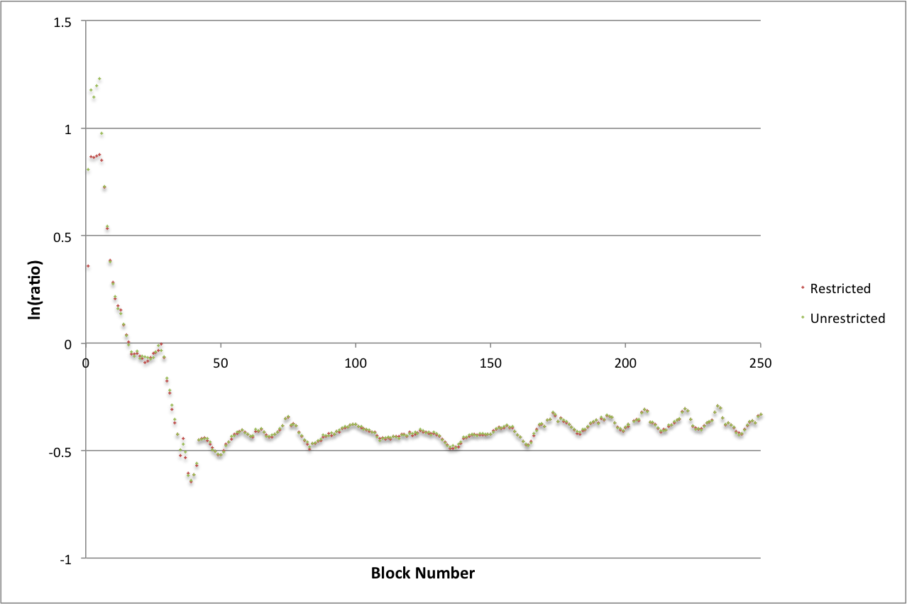
Figure 2: Comparison of the performance of the restricted and unrestricted pressure calculations
In Figure 2 one can see that after about 10 blocks the time taken by the run with a restricted number of iterations coincides with that of unrestricted run. This suggests that the runs are producing very similar results - a conclusion that has been confirmed by examining the physical results in more detail.
In summary, this project has achieved two of the three planned objectives, and the third is being carried forward under an EPSRC research grant. By replacing the existing bespoke Jacobi/SOR pressure solver with a a Krylov Subspace method from the PETSc library, and implementing a number of optimisations to both MPI and OpenMP in the code, we have been able to to speed up calculations on a physically relevant grid size (11 million elements) by over 50% in the pressure solver alone. We have also demonstrated excellent strong and weak scaling of the code well beyond 20 million elements.
Our investigations of the behaviour of TPLS have led to several suggestions for further work. The most urgent need is for the current serial I/O strategy to be replaced by parallel I/O (for example as described in [3]), as this is a significant bottleneck to further scaling and currently takes over half the runtime for the calculations we have used for testing. In addition, the other main computational parts of the code - the momentum and interface solvers - would also benefit from being ported to PETSc. As well as giving a direct performance increase, this would remove the need for frequent copying between PETSc and TPLS data structures, reducing time and memory overheads, and also allow the flexibility to move to a full 3D domain decomposition. Thirdly, we believe that using multi-grid preconditioners may give further speed improvements in the pressure solver. Working versions of these are available in PETSc 3.4, which we have not yet been able to test.
Finally, as a direct result of this dCSE project, we have made the entire TPLS code available under the open-source BSD license. The code can be downloaded from https://sourceforge.net/projects/tpls/ and as we continue to develop and improve TLPS we hope to grow a community of users and developers who can now take advantage of our work.
This project was funded under the HECToR Distributed Computational Science and Engineering (CSE) Service operated by NAG Ltd. HECToR – A Research Councils UK High End Computing Service - is the UK’s national supercomputing service, managed by EPSRC on behalf of the participating Research Councils. Its mission is to support capability science and engineering in UK academia. The HECToR supercomputers are managed by UoE HPCx Ltd and the CSE Support Service is provided by NAG Ltd. http://www.hector.ac.uk.