Improving Performance of TOMCAT for High Resolution Simulations

 

 

Dr. Mark Richardson, Numerical Algorithms Group

Professor Martyn Chipperfield, School of Earth and Environment, University of Leeds

 

 

 

 

Abstract

TOMCAT is simulation code for atmospheric chemistry and transport processes. It operates in distributed memory mode with an option to activate shared memory parallelism. The performance of the code when simulating high resolution cases has been investigated. A concern is that the file access pattern will affect the performance due to the increase in data volume being read-from and written-to file storage.

The raw performance of the code has been shown to be the best it can get, with one routine dominating the calculation phase using 50% of the time per iteration. However, the areas of weakness lay in the file access patterns. This analysis shows that although the actual cost of writing and reading data is small, the supporting features of data collection prior to writing and data distribution post reading are not efficient.

Four functions were chosen for improvement and two of these demonstrated dramatic improvements in performance. For example, a function reporting altitude profiles of a calculated field added an overhead of as much as 40 seconds in its original form. The revised version is less than 0.05 seconds overhead on the iteration. The second two functions are not currently widely used, but the revised versions can be used elsewhere in the code as replacements for other  functions.

 

 

Improving Performance of TOMCAT for High Resolution Simulations. 1

1        Introduction. 3

2        Task 1.1: Analysis of the Existing Software. 3

3        Task 1.2: Restructure code to improve performance. 5

4        Task 2.1: Parallel-IO.. 6

4.1      Background for parallel IO task. 6

4.2      Reporting Ground Based Station Profiles. 6

4.2.1     Overview of the current implementation. 7

4.2.2     Method for new version. 7

4.2.3     Memory Requirement and Some Alleviation. 8

4.2.4     Communication Analysis. 8

4.2.5     Summary GBSTAT. 8

4.3      Evaluating Zonal Mean for a Calculated Quantity. 9

4.3.1     Overview of original implementation. 9

4.3.2     Method for replacement of SORZM... 9

4.3.3     Memory Requirement and Some Alleviation. 10

4.3.4     Communication Analysis. 10

4.3.5     Summary SORZM... 10

4.4      Improved Gather and Scatter 11

4.4.1     The need for bespoke data types. 11

4.4.2     File reader PPREAD is replaced by PPRD.. 12

4.4.3     File writer PPWRIT is replaced by PPWR.. 13

4.4.4     Development of the parallel file access model 13

4.5      Summary of Task 2.1(Parallel IO) 13

5        Analysis of NetCDF features. 13

6        Project Conclusion. 14

7        References. 14

 

 

 

1         Introduction

This project was funded under the HECToR Distributed Computational Science and Engineering (CSE) Service operated by NAG Ltd. HECToR – A Research Councils UK High End Computing Service - is the UK's national supercomputing service, managed by EPSRC on behalf of the participating Research Councils. Its mission is to support capability science and engineering in UK academia. The HECToR supercomputers are managed by University of Edinburgh, HPCx Ltd and the CSE Support Service is provided by NAG Ltd.

This project was undertaken to support the development of the TOMCAT atmospheric process simulation code (www.see.leeds.ac.uk/tomcat). This report details the analysis performed on a high resolution model. The time per iteration and Cray performance analysis tools are used to identify places in the code where changes might lead to improving the time for simulation runs. The changes might also lead onto improved scalability. This final report describes the work undertaken for four tasks; analysing the behaviour of the code for the high resolution model, reporting the changes made to improve the raw performance, modifying the way in which TOMCAT interacts with files and reporting on the NetCDF features that had been incorporated only a short time before this project was started.

The current Phase 3 of the HECToR system (a Cray XE6) has 5632 AMD Interlagos processors and is described in detail on the hector public web site: www.hector.ac.uk. The significance is that earlier TOMCAT projects took place on different phases of HECToR and working practices were matched to the hardware. For example, spacing out MPI tasks to underpopulate nodes but then use OpenMP parallelism to use the otherwise idle cores. Phase 3 of HECToR uses the Cray Gemini interconnect for routing communications between processors but the memory per core is now 1GB.

Cray PAT tools have been used to analyse a limited number of steps of the simulation (96). Timing and analysis has been done for three different MPI decompositions (80, 160 and 400 MPI tasks). The code provides some raw timing derived from calls to MPI_WTIME and these have guided the research to where the workload is highest. A facility in Cray PAT, for tracing file access, has been used to determine the amount of data being read-from, and written-to, various external files throughout the simulation.

The TOMCAT software is a chemical advection transport code. It processes chemical and aerosol data to provide the time evolution and distribution of chemical species around the whole earth atmosphere. The T42 (2.8° x 2.8°) case was used in previous DCSE work [1]. That effort improved the performance of TOMCAT by some restructuring of key routines and modifying some of the functions that prepare data for MPI communication. In a second DCSE [2], OpenMP was added to help improve the time for simulations by reducing the number of MPI tasks per node and utilising the “idle” cores by sharing the work of five loops over the remaining idle cores. The result was that using four OpenMP threads with one MPI task per NUMA node made the use of 128 cores more efficient than using 128 MPI tasks directly.

This project has used the high resolution model of T106 (1.2° x 1.2°). It was supplied initially with decomposition for 80 MPI tasks for the “high resolution” situation. Although this is referred to as the “1-by-1” it is actually 320 by 160 grid-boxes of 60 layers, thus not quite 1 degree intervals but approximately nine times more computational cells than T42.

2         Task 1.1: Analysis of the Existing Software.

The first task has been to establish the performance profile of this version of the software with the high resolution case. A couple of methods are available; one is the user-defined timing reports and the other is the use of Cray PAT. The latter was further refined by selectively turning on the recording of the performance data. More detail is provided in the progress report [3] delivered during the course of this project.

The source code contains calls to MPI_WTIME so that elapsed time and time per iteration is reported. Examination of the timing reports reveals that the time per iteration is not uniform and for some of the iterations the elapsed time is as much as fifteen times greater than the time taken for the majority of iterations.

Table 1 shows the raw performance before any enhancements. It includes OpenMP parallelism as well as the MPI scaling information. The majority of this project work used only single-threaded MPI configurations. The variation in elapsed time per iteration, for a given configuration, is due to several factors: the cyclic reading of reference data, the initialisation and the completion of the simulation. The flexibility of the program includes the possibility of writing data on a regular basis for post processing.

 

Table 1: Baseline effect of OpenMP on three MPI configurations. Six stages of simulation are distinguished.

 

Where scaling is concerned the time ‘per step’ (intermediate step) reduces in a non-linear manner as the numbers of MPI tasks are increased. There are also sections of the simulation over which the time taken does not vary with the number of MPI tasks. They are likely to be where significant output is being done. The experiments were done with the MPI tasks spread out over the nodes such that the placement was one MPI task per 4 cores (the “-d 4” option for aprun). This allows OMP_NUM_THREADS to be modified to 1, 2, 3 or 4. Thus there is a possible 4GB of memory available per MPI process, similar to the first phase of HECToR.

This simulation executes 96 iterations, in which it can be observed that the first iteration is approximately 330 seconds wall time for all MPI configurations and that each of the intermediate iterations is in the case with 80 MPI tasks is 1 second. Thus an overall runtime of ~450 seconds wall time is recorded as a baseline. The scaling is clearer when considering an intermediate “interval” step. i.e. one where there is minimal or no file access.

At this resolution the application retains the OpenMP threads scaling characteristic that it had at the lower resolution, in the work done for implementing the hybrid parallel operation. In production use the simulation could be decades, needing of the order 3650x96 iterations. Some features that appear significant within the 96 iterations of this investigation might not have the same impact for a production run.

The perftools module has to be activated so that the code can be instrumented. The tools help to identify regions of high workload and to track file interaction. There are many ways of using the tools with those shown in figure 1 being the main methods applied in this project task.

 

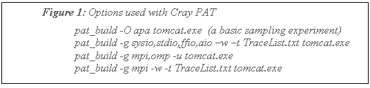
Cray PAT has been used to inspect the runtime behaviour of the software. Sampling experiments are used as an initial pass to confirm the routines which will be investigated further. Trace experiments are used with tracing focussed on those identified subroutines plus any other routine that showed up in the sampling experiment. Additional experiments were done using the “io” group function which reports the volume and rate of data being read from and written to external files.

Intermediate iterations are of short duration by wall time so by default very few samples are recorded. Refined analysis can be achieved by controlling when the tools record the data. The sampling rate can be increased by shortening the sampling interval. This allows a significant number of samples to occur while the PAT record is active. The default interval (PAT_RT_INTERVAL) is 10000 (i.e. 10 ms) so setting it to 100 microseconds should provide 10000 sample in a 1 second wall-time interval. There is an API for defining regions of interest. In the file, that is the log of the instrumented run, the number of samples are (or time spent is, if it was a trace experiment) attributed to those regions. Increasing the sample rate will slow down the experiment and produce larger logs.

The “pat_record” feature was used to choose where to activate the sampling or trace information. Using the information from the sampling experiment, the recording was activated in each of the zones of interest and several repeat runs were done for different recorded regions. A call to pat_record is made at the start of the program so that the recording is turned off. At a pre-determined point it is switched on and for one step the profile is recorded. This reduces the amount of data collected but the program is still slower as it is continuously sampling at the higher frequency to capture the occasions when the code enters the regions of interest.

Restricting the recording to single iterations of interest reveals differences in workload. For the intermediate iteration (“standard” time step without special processing) as much as 50% of the wall time for the iteration is spent within CONSOM, some time was spent trying to improve that function.

3         Task 1.2: Restructure code to improve performance

The CONSOM subroutine has been identified as a high work load function and this section describes its structure. It is a function for mixing tracers by convection. Historically the subroutine has accessed files, which explains the code structure. Usually the developers organise the loop structures with the outer loop for the final index in the array dimensions (the longest stride through memory). For this subroutine the outer loop is for the latitudes (the second index). The rationale is that the convection terms per latitude could be stored on disk after they had been calculated. The calculation still adheres to that structure working in planes of altitude and longitude for all tracers before moving on to the next latitude. The innermost loops do cycle through the first index (of contiguous data) for longitude.

A switch for the compiler to give information about how it is compiling each subroutine was enabled and revealed the following output shown in figure 2 (note the highlighted bold text). The compiler typically complains that there are too many levels of nesting of DO loops. It also seems to want to rearrange the order of calculation of loops I and L. This is because the access of the coefficient matrices is invariant with altitude but varies with longitude.

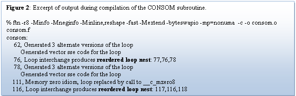
Re-writing the code to match the compiler optimisations and then re-compiling provided similar messages but this time nesting the loops to the original order. Following this detailed analysis it was concluded that the only way to enhance the performance of CONSOM would be to introduce hardware-specific tuning such as cache line blocking of loops. However, the benefit is not a clear advantage considering the work required and portability.

4         Task 2.1: Parallel-IO

4.1       Background for parallel IO task

In this section four specific features that interact with external files are analysed, revised and reported. Three write data and one reads data. Two of the writers, GBSTAT and SORZM, have almost identical features in terms of data storage and data communication. The other writer (PPWRIT) is very similar to the reader PPREAD except the process is done in reverse.

The function GBSTAT is for reporting information at the longitude and latitude of “ground based stations” although in contemporary use this can mean any location where empirical data has been acquired (i.e. this includes shipborne or airborne experiments). The function SORZM, evaluates the average of the circumferential values of specific scalars (i.e. along lines parallel to latitude) and stores the result in a meridian plane. They both contain “Gather” style functionality although in one case the gather is ahead of several interpolations and for the second the gather is ahead of the latitudinal summations. These gather operations are expensive as they involve transferring the whole field of interest onto the MPI task zero (in fact several fields are processed this way).

The function (PPREAD) occurs during initialisation of the experiment and follows the policy of a master task file reader. The fourth (PPWRIT) is used for writing data to files. These two functions are in fact a serial reader and a serial writer but additional complex wrappers are integrated to perform distribution to (after a read) and collection from (before a write) the other MPI tasks by MPI task zero.

The next three sub-sections give detail of each function with analysis of the existing method followed by the description of the replacement method. Greater detail can be found in the reports that were provided to the lead developer during the progress of the work [3], [4] and [5]

4.2       Reporting Ground Based Station Profiles

The function GBSTAT is likely to be activated for specific cases with output on each 6 hour cycle (e.g. 24 steps). Also, different simulations will output data at a different number of ground-based stations. Some experiments might save data at around 300 sites with up to hourly frequency.

For this work the GBS reporting has been artificially activated for every other time step (each half hour) and highlights the weakness of the existing method. An indicator of the changes is shown in table 2.

4.2.1     Overview of the current implementation

The algorithm has four sections; in the first section there is a loop over tracers and field data in which they are transferred to the master MPI task zero, it has to store them in a global-sized three-dimensional array. The second is where task zero searches the global data to find four surrounding data points for interpolation, so all other MPI tasks are idle. The third section performs the interpolation on task zero and the fourth section writes the interpolated values to a file from task zero. This subroutine demands significant volume of data to be communicated to process zero and the interpolation is done solely on that root process.

4.2.2     Method for new version

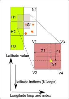
The Cray PAT analysis indicated that the file writing takes a very small amount of time compared to the rest of the subroutine so the serial (master-io) has been retained for compatibility. Each MPI Task determines whether it contains any ground based station. If there are any, it should evaluate the field variable at the interpolated location and report the column of data back to the root process. Special treatment would be needed near edge of a patch except the halo region is updated ahead of the interpolation. When the ground based station is within a grid-box on the boundary of a patch, it could be that a number of straddle points are on another patch. A temporary array is declared that includes a halo and the field data is copied into the local temporary three-dimensional array. All patches will communicate their shadow data to adjacent patches that then copy this into the temporary array.

Figure 3: The bi-linear interpolation used in both methods, indicating the need for halo updates.

The report of the interpolated values to MPI task zero is done in a parallel gather. The local storage is small, but large enough for the case where all GBS are on one patch. The storing of the locally calculated profile is placed in the appropriate storage location on the gathering task (corresponding to the GBS ID). The collecting MPI task will write in the usual serial manner to retain compatibility. Compared to the original method only the final collection and write to file are done on task zero and thus the non-writing tasks are idle for less time.

4.2.3     Memory Requirement and Some Alleviation

The removal of the transfer of all local fields back to task zero removes local storage of approximately 330 Mbytes. There is a need for some extra temporary storage in the form of the array that includes halo storage for a local array and the buffers that transfer the shadow data to the haloes on adjacent PEs. The amount of memory added is only 70 Mbytes. The net benefit is a reduction of 260 MBytes for this function.

4.2.4     Communication Analysis

There is no longer a need to transfer all the local field data (per tracer) to task zero which reduces the communicated data by 280 MBytes. The need for updating the halo region for all MPI tasks adds 70 MBytes and this is simpler than adding “intelligence” for determining which tasks need halo. This amount varies with the decomposition the number of tasks determines the number of interfaces. The net effect is that the communicated data is reduced by 210 MBytes.

4.2.5     Summary GBSTAT

The improvements to this subroutine have made the related experiments significantly cheaper. Some of this is attributable to the parallelisation of the process and some will be due to the lower memory footprint of the task (previous work showed that spacing out the MPI tasks results in improved performance due to memory issues).

The table 2 shows that there are significant changes to the writing step that result in a dramatic reduction in the cost of writing the ground based station profiles.

 

Figure 4(a). Standard method.                        Figure 4(b). Modified method.

 .

 

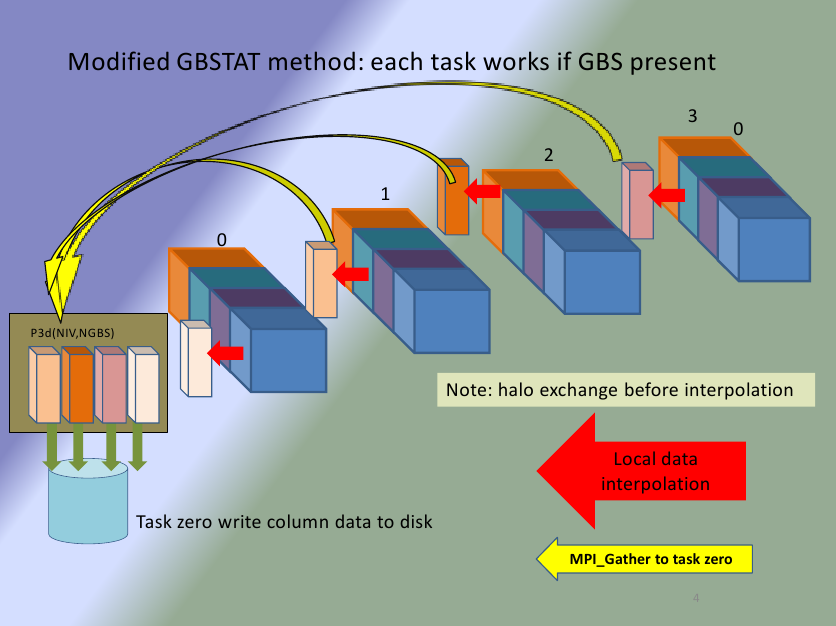
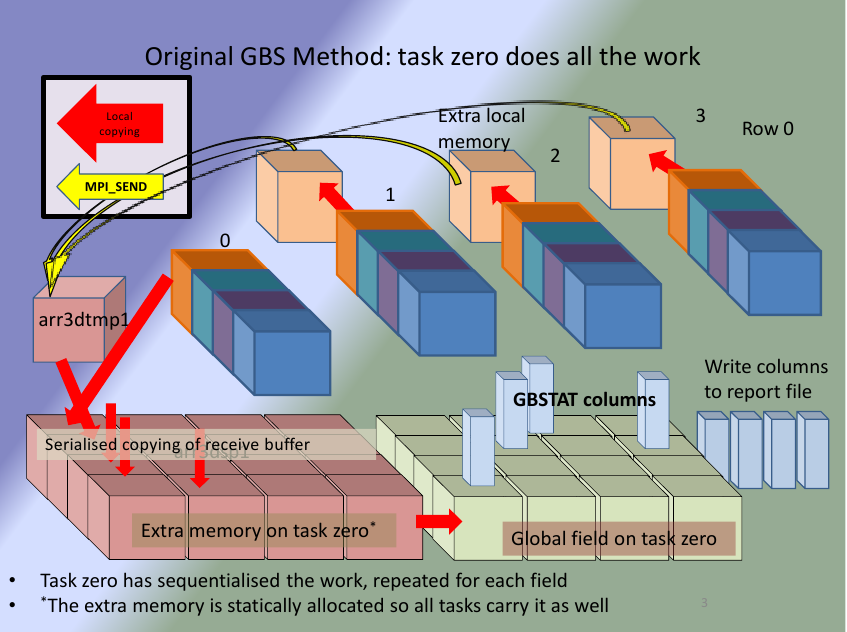
Figure 4(a) shows the collection of one field of data for only the first row of MPI tasks. The 16 large cube shapes, arranged in rows of 4 in the diagram, represent storage for the distributed field data. There are four individual cubes that represent the send buffers on each of the MPI tasks in the top row of the task topology. The two groups of sixteen blocks at the bottom of the diagram are the extra storage required; one for assembling the incoming buffers and the second for the field calculation. Due to the single program-multiple data philosophy and static arrays the storage is repeated on all MPI tasks putting a high demand on the memory sub-system of any shared nodes.

Figure 4(b) is the modified method and illustrates the reduced amount of storage for the equivalent of the process in figure 4(a). The process has been greatly simplified and leads to a method that can be easily maintained and adapted if need arises.

4.3       Evaluating Zonal Mean for a Calculated Quantity.

4.3.1     Overview of original implementation

The function SORZM evaluates the zonal mean for several species. It broadly follows the methodology of the function GBSTAT. The field of data on a patch is copied to process zero. This is achieved by copying the local data into a temporary array equal to the size of the local data set. The reference locations of the sub-domain are sent to the master task and then the local copy is sent using MPI_SEND to the master MPI task (task zero). The zeroth task copies this buffer into the corresponding location of a globally sized data array. Task zero then sums the values along a line of latitude. This is done within the longitude loop and then below a species loop. The calculation of the average is simply division by the number of contributing values, i.e. sum(1:NLON)/NLON. The master task then writes the data to file. Thus the structure of the file is per species around planes of longitude by latitude. The process is shown diagrammatically in figure 5(a).

4.3.2     Method for replacement of SORZM

In the revised method, the values along a line of latitude within an MPI task are summed together into a two-dimensional array, equivalent to the west-most face of the computational space. This is a similar method to the original but the data being summed is all local data so all MPI tasks are busy working with their information simultaneously. Then, using MPI reduction, these “planes” are summed along a row of MPI tasks. The communication is minimised by not using MPI_Reduceall so the final sum is stored only on the MPI task that is “root” for the row (the zeroth rank of the row of PEs). A separate communicator for each row is used to ensure the sum is done on only relevant MPI task data. The zonal means are evaluated and then recovered to process zero with MPI_GatherV. The result is then written to the usual file, it is important that this in the order that matches the original version. The main reason for retaining this feature is to keep the file identical to the one produced by the original method. An alternative method is to allow each “row-master” to write its section to the file in parallel as this would reduce the time of the write and avoid the collection to MPI task zero. That would require MPI-IO functions and the output format would be of the “stream” variety and thus difficult to compare with the original version. A diagram of this process is shown in Figure 5b.

The average values are potentially different to those seen in the serial version. The serial method adds up the values around the line of latitude in ascending order of longitude. When the values of a variable that vary in order of magnitude are accumulated in different sequence it may be that the final value will not be the same for each case where the order is changed. Adding a large number to a small number might be at the limit of precision of the machine but accumulating lots of similar sized values may eventually result in a large value that can be added to a large value. A method known as “binning” could be used where accumulators work with similar sized numbers until eventually the final result is present in a single “bin”. Similar problems occur when adding numbers of opposite sign. A large negative number added to a large positive number might not result in zero even when on human inspection they should.

4.3.3     Memory Requirement and Some Alleviation

The estimated reduction in storage requirement for this method is 330 MBytes which is due to the removal of the globally-sized storage and copies of several multi-dimensional arrays. A certain amount of temporary storage is still needed for buffers and the communicated sums which add approximately 1 MBytes. Thus the net change in storage requirement is a reduction of 329 MBytes.

4.3.4     Communication Analysis 

In the original method the full fields are sent to the root MPI task. For the configuration using 80 MPI tasks that is 280 MBytes data transferred. In the revised version the smaller quantity of data in the end planes is communicated instead, less than 1 MBytes. These planes will vary in size according to the number of MPI tasks. However, the data that is being summed remains the same for this resolution of model as the number of tasks in the latitudinal direction remains the same (five columns). The net reduction is thus 279 MBytes.

4.3.5     Summary SORZM

Table 3 shows the difference in timing of the iterations for writing and not-writing the information. Previously, the overhead of this function increased significantly (10x) when more MPI tasks were used. The new method is less than 10% of the time step even when the larger number of MPI tasks were in use.

The improvements to the function for calculating zonal mean have made the feature less expensive and thus a researcher can consider increasing the number of times that they ask for this data to be logged. A time series plot of such data could reveal trends that might have been missed when using a lower frequency output.

 

Figure 5(a): The original method for zonal mean.       Figure 5(b): Modified method.

             

 

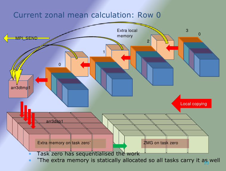
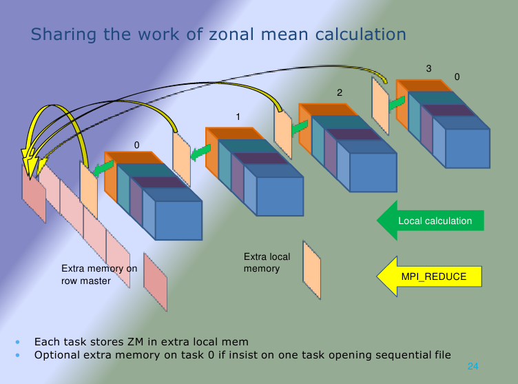
In a similar manner to figure 4, the figures 5(a) and (b) have been provided to illustrate the difference for one row of the MPI topology. The memory requirement has been greatly reduced as it was for the GBSTAT work.

4.4       Improved Gather and Scatter

4.4.1     The need for bespoke data types

The MPI intrinsic functions require the type of the data to be specified in the calling interface. The number of data types that are pre-defined in MPI are limited (although approximately 64 can be seen in the system’s mpif.h include file). These fundamental data types can be used as a foundation on which to build user-defined data types where the data structures are more complicated than a vector of the foundation data type.

The computation is done in parallel by decomposing the rectangular computational space into a two-dimensional grid of sub-domains. This is clearly defined ahead of the simulation and does not change during the simulation. The existing code uses “DISTF” to scatter data that has just been read. The function involves significant data movement: first, parts of the array are copied into per-process buffers and then a loop is used to cycle around each MPI task in turn with an MPI send function. This is unfortunately serialising what could be a more efficient task handled by the system layer of MPI.

Three custom data types are very useful to use instead of this arrangement. They are columns of contiguous data arranged into the computational blocks; in one case the data types include storage for halo data and in the second case the data type does not have any, nor allow for, halo storage. This matches the types of variable used in TOMCAT calculations as some need halo data and some do not need halo data. The third data type is formed from several columns without halo. The columns make up a planar component for a sub-domain. It is useful where data scattering is used as only the internal points of the global-sized array are distributed to the local two-dimensional arrays. When a data type is “registered” with MPI much of the buffer copying is shifted into the MPI layer. The definitions are done within Fortran modules and the data types are therefore global.

 

Figure 6: Schematic demonstrating new data types used with MPI_ScatterV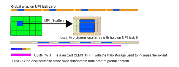

 

Figure 6 shows that shaded sections of the global array on task zero form a coherent rectangle of data that is needed on MPI task 6. The receptacle on the distributed task is a local two-dimensional array with halo storage.

The MPI_ScatterV function is applied to the data on a “root” task and distributed to all tasks that share a communicator.

 

 

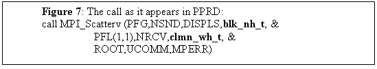
The scatter makes it possible to send the block fragment of the global array PFG (on task zero) to be received into a number of columns of local two-dimensional array, PFL, which has storage for halo data. In the existing code a flag is used to indicate the halo requirements of the communicated array. This level of indirection is removed because the data type replaces this need for a conditional flag and the copying functionality of DISTF is now taken care of by the MPI layer as seen in figure 7.

The multi-dimensional data is referenced in planes and within a plane the two-dimensional structures are unwrapped into one-dimensional vectors. These work well with the foundation data types of MPI. However, there are a lot of user-defined interventions and re-arranging of the data to get to the vector state.

4.4.2     File reader PPREAD is replaced by PPRD

The existing version of TOMCAT includes a pseudo-parallel reader “PPREAD” that is actually a serial reader followed by a call to their distribution function, DISTF. The existing implementation of the PPREAD function converts the two-dimensional plane into a vector of elements, reshaping at the interface (rather than a formal re-shape of the array into a vector ahead of the call). It then reads the whole plane from file, which is passed to DISTF which converts the one-dimensional vector into a two-dimensional array. This is then copied into a buffer with an entry per MPI task so that the re-packed array can be sent to each MPI task in turn. Each MPI task then copies the buffer into the local working two-dimensional array.

The calls to DISTF allow for the variation in size of the receiving array, it is called with different arguments to indicate the extent of the data as shown in figure 8. In one case the size has no space for storing halo data in the second case it allows for storage of halo data. This allows the unpacking function to populate the vector in an array manner with holes where the halo information is stored.

 

 

Within DISTF the PFG storage is copied into a buffer that stores data according to destination MPI task. When the send-receive sequence (note it is a sequence in this implementation) has completed the received vector is unpacked into PFL as described above. On the return to the calling function PPREAD this vector is re-shaped (through the interface) into the two-dimensional local array ready for use on the MPI task. This can be classed as “user-programming” and is not the most efficient use of the system MPI implementation. The mapping from the global two-dimensional array into local two-dimensional arrays can be achieved user-defined data types as described in the previous section.

 

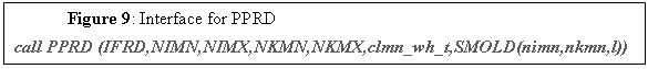
The replacement function PPRD does not use DISTF but refers to the matching data type for the array being read from file. As a consequence it requires the extent of the array as shown in figure 9.

4.4.3     File writer PPWRIT is replaced by PPWR

In a similar manner to PPRD, the function PPWR replaces a user defined “Gatherer” (COLLF) to collect the distributed field onto MPI task zero ahead of writing to an unformatted file.

In the original algorithm COLLF has a barrier at the start (this is some legacy solution to a problem that is unlikely to exist if the new technique is used). The local field information (excluding halo information) is loaded into a buffer that is sized to take the whole plane of the global plane but arranged by processor. In the subsequent conditional structure the MPI task zero receives each of the sub-planes in turn. All the other MPI tasks send their individual plane (a slice of this large buffer) to the master task. The significance of using the large buffer is that, as it exists on all tasks, it is filled in a safe fashion per MPI task on task zero. There follows a decoding session where this received buffer is unpacked into the global field array.

4.4.4     Development of the parallel file access model

The prototypes that have been prepared to extend this work allow the serial form of master IO to be enhanced to row-master file access for reading or writing. Changes will have to be made to the data structures in the existing reference data files. This is because it has become clear that the existing method reads (and writes) a whole plane of data and thus “end-of-record” indicators do not align with the latitudes that would be used for parallel reading.

If the records of the external file had corresponded to individual latitudes then the access could have been restricted to the number of latitudes in-common with the range of latitudes on the “row-master”.

4.5       Summary of Task 2.1(Parallel IO)

In this section, the four functions (GBSTAT, SORZM, PPREAD and PPWRIT) were chosen as extreme examples of what can be achieved. In the first two functions significant re-writing has resulted in significant gains, when those functions are activated. Already the new method has been re-used within a function that deals with satellite data. In that situation there are 15 samples a day at differing longitude and latitude, so a low-cost algorithm is important.

The second two functions did not demonstrate immediate performance improvements, as their use is not as extensive as it could be. Also the developments of those will not be at their most useful until the file data structures become aligned with latitudes. The user-defined data types are now available for future use by TOMCAT developers and the replacement PPRD and PPWR can be used in other places in the code. For example in DEEPTDINI, DEEPTDINT, OZNINI, OZNINT, STINI, STINT, TSINI and TSINT.

In all four replacement algorithms the underlying serial file access method has been retained for compatibility and thus makes them immediately available for use in production work.

5         Analysis of NetCDF features

The version of the code used for this project included a development version of NetCDF functionality.

FINITER is where the decision is made to use NetCDF or the unformatted Fortran binary write. The sequence of calls is: INICDF, INI_DIAGCDF and WRITE_CDF. The two initialisation routines are only processed on the first pass. The writer is called at the end of each iteration as requested by the user.

INICDF : a file is created and the full set of variables is defined. Some meta-data is processed (i.e. invariant for the simulation but varying between simulations).

INI_DIAGCDF : this is for a corresponding diagnostics file written at the same time if the diagnostics mode is selected.

WRITE_CDF: the actual writing of specific variables. It is a complex subroutine with a lot of processing that is confined to task zero. This is the same “serial writer” approach that is taken in the original GBSTAT, SORZM and the PPWRIT functions. The method requires the collection of the full data volume onto one MPI task before the processing and writing to file. Other functions that use a collector include PUT_CDF_VAR3D, PUT_CDF_VAR2D, PUT_CDF_VAR2D_INT and MONTHLY_MEAN.

There is a clear possibility of improving this feature by two methods changing the process of gathering and optionally not gathering the data directly but using “parallel NetCDF”. The new data types provide mechanisms for the former whereas more work is required for the latter by removing all the filters and collectors. A choice has yet to be made.

6         Project Conclusion

The work for this project has shown that the core function is already at its best performance. The core of the code is in good health and would require hardware-specific tuning to make further gains. What were perceived as file access bottlenecks were in fact the attendant processing for reading and writing data. Significant refactoring has changed the performance profile of the file access sections of two functions in the code. The changes have made those features almost undetectable in the per step timing information.

User-defined data types have been implemented that can be used anywhere in the code that needs to gather data for writing or to distribute data after reading. These should be used in preference to “re-inventing the wheel” for any future developments.

A version of this report has been presented at the Cray User Group Meeting in May 2013.

7         References

[1]     M.Richardson, “Improving TOMCAT/GLOMAP Mode MPI for Use on HECToR, a Cray XT4h system”, HECToR DCSE programme, www.hector.ac.uk , April 2009.

[2]     M.Richardson, G.W.Mann, M.P.Chipperfield, K.Carslaw, “Implementation of OpenMP within MPI-TOMCAT-GLOMAP mode”, Cray User Group Meeting, Edinburgh,  May 2010. (also full report available on HECToR web-site).

[3]     Progress Report 1: M.Richardson, M.P.Chipperfield, “Performance Characteristics Of TOMCAT For High Resolution Simulations”, HECToR DCSE programme, www.hector.ac.uk , October 2012.

[4]     M. Richardson, Progress Report 2: Modification of GBSTAT, March 2013.

[5]     M. Richardson, Progress Report 3: Modification of SORZM, May 2013.