A necessary side product of the conversion of the SWT code to use FFTW was a routine to carry out Chebyshev transforms. Had the FFT API of 2DECOMP&FFT been used, it would have been necessary to incorporate this into that library; as it stands, the domain decomposition API was chosen instead, so this is not necessary. However, it was considered appropriate to adapt and generalise this routine so as to make it suitable for use in or with 2DECOMP&FFT. This would broaden the capabilities of this library by reusing a side-product of this project.
Given a function ![]() on the interval
on the interval
![]() , and making a change of variable
, and making a change of variable
where
![]() , we define
, we define
![]() .
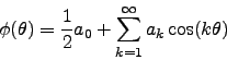
. ![]() can be
expanded in a cosine series
can be
expanded in a cosine series
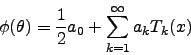
The Chebyshev polynomials ![]() of the first kind are defined
of the first kind are defined
so
Note that the coefficients ![]() in 13 and 15 are the same.
It is, therefore, possible to obtain them using a cosine transform, computable with
the FFT algorithm. It is also possible, with some manipulation, to use a standard FFT.
The SWT code originally used a complex-to-real FFT for this
purpose, and Chebyshev transform routines in
in 13 and 15 are the same.
It is, therefore, possible to obtain them using a cosine transform, computable with
the FFT algorithm. It is also possible, with some manipulation, to use a standard FFT.
The SWT code originally used a complex-to-real FFT for this
purpose, and Chebyshev transform routines in ![]() ,
, ![]() and
and ![]() (or rather the array indeces
usually corresponding to those dimensions) were developed from this. However, as
FFTW3 supports cosine transforms, an alternative set of routines was created taking
advantage of these. Both sets have been made available to
Dr. Ning Li, the developer of 2DECOMP&FFT.
(or rather the array indeces
usually corresponding to those dimensions) were developed from this. However, as
FFTW3 supports cosine transforms, an alternative set of routines was created taking
advantage of these. Both sets have been made available to
Dr. Ning Li, the developer of 2DECOMP&FFT.
Collocation methods based on Chebyshev polynomials usually use the Chebyshev-Gauss points
located at the roots of ![]() , and given by
, and given by
or the Gauss-Lobatto points, located at the extrema of ![]() (in other words, at the
zero points of
(in other words, at the
zero points of ![]() rather than
rather than ![]() ). These are given by
). These are given by
For applications such as SWT - which is designed to simulate flow through a channel of
fixed depth - the Gauss-Lobatto points are preferred; the zeroth and Nth points are at
1 and -1, and do not depend, as the Chebyshev-Gauss points do, on ![]() . Both grids are
supported; at present, the default is to use the Gauss-Lobatto points, and an optional
argument is used (if present) to switch to Chebyshev-Gauss.
. Both grids are
supported; at present, the default is to use the Gauss-Lobatto points, and an optional
argument is used (if present) to switch to Chebyshev-Gauss.