Abstract

The RMT method (R-Matrix with time-dependence) is a new ab initio method for solving the time-dependent Schrödinger Equation (TDSE) for multi-electron atomic and molecular systems in intense short laser pulses. Although several other time-dependent R-Matrix methods have been introduced in recent years [1, 2, 3, 4, 5, 6], RMT demonstrates orders-of-magnitude improvements in efficiency, primarily because it employs finite-difference (FD) techniques to model the few-electron wavefunction far from the atomic core. RMT merges the Outer Region FD model with a classic B-Spline R-Matrix basis set for the multi-electron Inner Region [7]. The difficult problem of merging a basis set model with a spatially adjacent FD model, while maintaining the unitarity of the time-propagator, has been a long-standing barrier to progress in this field. RMT is based on the solution first published in 2008 by Nikolopoulos, Parker and Taylor [8].

In this report we discuss the implementation and testing of a new RMT code for calculating the spectrum of light scattered by atoms interacting with intense-field laser pulses. At sufficiently high laser intensities, atoms scatter the incident radiation not just at the frequency of the laser, but also at odd-integer multiples of the laser frequency. This process we refer to as High Harmonic Generation (HHG). The spectrum of light scattered in HHG processes is obtained directly from the Fourier transform of the time-dependent expectation value of the acceleration induced by the external light source (the laser pulse). The bulk of this project has been devoted writing new code to calculate these expectation values, and to the much more difficult problem of assessing its correctness.

High harmonic spectra provide rich information about the electronic structure of atoms and molecules, in some cases with unprecedented time and spatial resolution. Experimental research groups at Imperial College London, University College London and CLF have used the information contained in the high-harmonic spectra to probe the electronic structure of polyatomic molecules [13]. The group at Imperial College has also recently pioneered the PACER technique [14] to study dynamical nuclear interference effects in molecules on an attosecond time scale [15].

Of the various theoretical approaches to the study of high harmonic generation, RMT is particularly well suited because it naturally models multiple final states of the residual ion created during ionisation, each of which needs to be accurately accounted for throughout the calculation. No other computer code to our knowledge, except HELIUM, can generate these time-dependent solutions to high accuracy. Moreover, recent attempts at developing models that go beyond the single-active-electron approximation are strongly suggestive of a crucial role played by multi-electron dynamics in determining the HHG emission rates in multi-electron atoms [16], but such models are still unable to provide a quantitative description of HHG yields. The need for an accurate quantitative description of HHG from rare gas atoms in order to provide guidance for future experimental investigations is the motivating factor behind our objective to implement the coding to make possible the calculation of high harmonic processes in the RMT code.

Although high harmonic generation specifically in molecules is of particular interest to UK experimentalists at Imperial College London and elsewhere and a RMT description of this process in multi-electron molecules is an eventual goal, it is first necessary to implement coding to make RMT calculation of this process possible for multi-electron atoms. This is because the HELIUM code provides a suitable code comparator role for the atomic case, helping the correctness of the new coding to be established. In a later stage (outside the scope of the current project) the RMT atomic code will play a similar comparator code role when implementing coding for the high harmonic generation process in a RMT molecular code.

Over the last 5 years, remarkable advances in laser technology have enabled experimental study of matter-laser interactions with unprecedented time-resolution. Experiments can now be performed using few-cycle pulses of high-intensity Ti:Sapphire laser light at  800 nm wavelengths, and at Vacuum-Ultraviolet wavelengths (VUV) with pulses as short as  250 attoseconds. The creation of attosecond pulses in particular has opened up a new frontier in the study of ultra-fast electronic processes. Recent landmark attosecond spectroscopic measurements in a solid [9] have demonstrated that ultra-fast techniques can probe solid state processes occurring at the theoretical ultimate speed limit for electronics. Attosecond pulses have recently enabled the real-time observation of electron tunnelling in atoms [10] and Auger decay of inner-shell electrons [11]. Attosecond pulses have also enabled stroboscopic study of single ionisation events in argon [12].

The goal of RMT has been to enable theoretical analysis of recent experimental advances with a degree of reliability that would be impossible by competing methods. These include time-resolved studies of ionisation events in attosecond time-scales, studies of time-delays between the ejection of electrons in double-ionisation, inner shell excitations and decays in complex atoms, intense-field atom-laser interactions in the XUV limit using the new free-electron x-ray lasers, and harmonic generation in atoms and molecules.

In a previous distributed CSE project we demonstrated that the RMT method is both computationally stable and could be distributed over 1000’s of cores with good efficiency. Success was due to the use of a mature R-Matrix parallel code for the Inner Region, and the use of the HELIUM finite-difference code for the Outer Region [17, 18]. In this project, a significant fraction of the effort has been devoted to assessing RMT by comparing the results of large-scale RMT integrations of laser-driven helium with the results of identical numerical integrations using the HELIUM code. HELIUM [19, 20] is a finite-difference code designed to generate high-integrity solutions of the full-dimensional time-dependent Schrödinger equation (TDSE) for two-electron atoms or ions in intense fields. HELIUM has been in heavy use on massively parallel machines since the arrival of the original Cray T3D over 15 years ago. The two methods of integrating the TDSE, the R-Matrix based RMT and the finite-difference based HELIUM, could not be more different. As we will demonstrate here, the two methods give good agreement in a series of rigorous tests that exercise mainly the inner (R-Matrix) region of the RMT code. The tests focus on harmonic generation by a helium atom irradiated by extremely short (attosecond) intense-field UV laser pulse and optical laser pulses. The good agreement observed between the two algorithmic methods helps to confirm that the methods and implementations are basically sound.

Contents

1 Objectives and Outcomes

In section 2 we discuss the goals and outcomes of Work Package 1, and we present the results of a significant test of the new code (as outlined in Work Package 3). The objective of Work Package 1 was to develop and test new RMT code for the calculation High Harmonic Generation (HHG) - the light scattered and shifted to higher frequencies by atoms interacting with intense laser radiation. The relevant Work Package 3 test is a comparison of two RMT calculations of HHG, the first derived from acceleration expectation values and the second derived from dipole expectation values. The two approaches are found to give good qualitative agreement over a 9 orders of magnitude range. Additionally we present measurements of the new RMT code’s scaling properties on HECToR, using a small 1-state helium-atom RMT calculation on a range of 34 to 1120 HECToR cores. We note that RMT calculations in more complicated atoms like neon would likely require an order of magnitude larger core count for both the inner and outer regions.

In section 3 we discuss the goals and outcomes of Work Package 2, and we present the results of one of the tests of the new code (as outlined in Work Package 3). The objective of Work Package 2 was to perform the same set of enhancements to the HELIUM code that were developed for the RMT code as described in section 2. The relevant Work Package 3 test is the same as the one described in section 2 for the new RMT code, a comparison of the high harmonic spectrum derived from acceleration expectation values with that derived from dipole expectation values. In HELIUM there is only one region, so no additional MPI communication software was required, but the integration is over two electrons (6 dimensional) instead of one, requiring a more laborious calculation of dipole expectation values < ψ(r₁,r₂,t)|z₁ + z₂|ψ(r₁,r₂,t) > , and acceleration expectation values < ψ(r₁,r₂,t)|dp₁∕dt + dp₂∕dt|ψ(r₁,r₂,t) >. We demonstrate that HELIUM HHG calculations based on acceleration expectation values and on the dipole expectation values give good qualitative agreement over an 11 orders of magnitude range.

In section 4 we discuss the goals and outcomes of Work Package 3. The objective of Work Package 3 was to test and tune the new code developments for numerical correctness and accuracy. Two of the more rigorous tests were discussed in sections 2 and 3. These two tests verified that the dipole expectation values and acceleration expectation values yield agreement in HHG calculations. In section 4 we continue with a series of tests that compare the predictions of RMT with those of HELIUM over a range of laser frequencies. We report good agreement between the two methods, which improves confidence in the correctness of the RMT code, and demonstrates that the RMT integration parameters have been properly tuned to produce numerical integrations comparable in quality to those of HELIUM.

2 Work Package 1. New Code for the Calculation of High Harmonic Generation (HHG) Processes

We begin with an outline of the basic RMT equations. The RMT wavefunction is the sum of an Outer and an Inner Region wavefunction. The Outer Region wavefunction is written on a finite-difference grid, and represents the single electron ejected from the atom by the laser pulse. The Inner Region wavefunction is described by a B-spline basis set. The Inner Region uses R-Matrix methods to treat the quantum mechanical dynamics of the multi-electron atom within a spherical shell of some fixed radius. In the following, that radius will always be 20 atomic units.

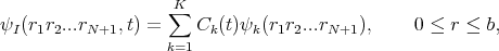
We write in the Inner Region I where all electrons can be found:

(1)

where ψ_k(r₁r₂...r_N+1),k = 1,K form a field-free, time-independent R-Matrix basis for the (N + 1) electrons within the Inner Region with outer boundary at r = b. The construction of the ψ_k is the responsibility of long-existing atomic R-Matrix time-independent codes. The time evolution of the Inner Region time-dependent wavefunction is entirely contained in the coefficients C_k(t) whose time evolution is determined by the TDSE. However in writing the TDSE we must take care that the Hamiltonian and dipole operators which act on ψ_I(r₁r₂...r_N+1,t) are Hermitian over Inner Region I (where ψ_I(r,t) is only defined). The Hermitian Inner Region Hamiltonian is given by H_I = H₀ + _h and the dipole operator by D_I = D + _d, where _h and _d are Bloch surface terms, only non-zero at r = b. In these circumstances the TDSE over Inner Region I is written:

(2)

where 0 ≤ r ≤ b.

This equation is a key one to the method. The second term on the right hand side compensates for the Bloch terms introduced to make H_I and D_I Hermitian. Note that it makes a contribution only at r = b and brings into play there ψ(r,t) a one-electron wavefunction form which we define from just within the Inner Region outwards. This term is central to any time propagation scheme in Inner Region I because it connects the wavefunction form ψ_I(r₁r₂...r_N+1,t) specific to that region with a wavefunction form that at r = b represents a single electron and which in calculations is obtained from Outer Region II.

The Outer Region II is spanned by a finite-difference (FD) grid so that the one-electron wavefunction there is written

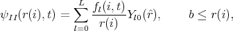(3)

with i = i_b,..,I and r(i_b) = b. In this form, for simplicity of presentation, we have allowed for only one residual ion state of the system. The form the TDSE takes in this Outer Region is then

(4)

This, the second key equation to the method, is the normal form of the TDSE over a FD grid except for the terms multiplying δ_iib and δ_iib+1. Note that these terms require quantities (the Bs) to be evaluated at grid points i_b - 1 and i_b - 2 i.e. at points on the inner side of the boundary at r = b. This assume we are using 5-point difference operators on the FD grid.

We emphasize how Eqs. (2) and (4) are actually used by sketching the computational procedure in propagating the full wavefunction through one time-step from t to t + τ. We first consider the Outer Region TDSE, Eq. (4). This is handled by the explicit Arnoldi time-propagator method [19] as in HELIUM and brings into play Inner Region information through the B_0l(i_b - 1,t), B_0l(i_b - 2,t) and B_1l(i_b - 1,t) terms all known from time t. Having thus determined all the f_l(i,t + τ) for i = i_b,..,I we proceed to the Inner Region. What we need to determine here are the coefficients C_k(t + τ) and again these are determined by the explicit Arnoldi time-propagator using knowledge of the Outer Region f_l(i,t + τ) to determine the spatial derivative terms at r = b brought in by the non-zero Bloch operator terms there.

Attempts to create efficient time-dependent R-Matrix integrations for such large volumes have made slow progress, largely because successful integration of the relevant high-dimensional partial differential equations is so computationally demanding that it requires the benefit of parallelization over tens of thousands of cores, which is not straightforward in pure R-Matrix formalisms.

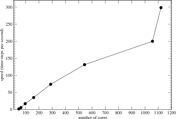
We turn now to a discussion of the scaling properties of the new RMT high harmonic generation code on HECToR. The performance and scaling of RMT is somewhat degraded by the additional computational overhead of the calculation of acceleration and the global MPI communications operations needed to complete, assemble and print the calculation of expectation values. To demonstrate the behaviour of the new RMT code, we choose parameters expected to be appropriate to harmonic generation problems in study of laser-molecule interactions. In these problems, the laser wavelengths are typically infra-red, and long in duration in order to resolve resonances with high accuracy. The numerical integrations in these cases require large integration volumes in order to accommodate the ionising electron during the duration of the laser pulse. By contrast, in a typical HELIUM integration at high (UV) frequency a small integration volume of 1000 a.u. might be used. In the present problem, figure 1, a volume of radius 3200 is used. The example shown in figure 1 uses a helium atom with a single target state for each possible final state angular momentum. The inner region Hamiltonian is a tri-diagonal block matrix, of size 32 x 32 blocks. Each block is a 55 x 55 matrix. A more complicated atom, like neon, or a configuration with more target states would likely require an inner region Hamiltonian one of more orders of magnitude larger.

The minimum number of cores needed to accommodate the inner region is 32. Using more than 64 cores provides no additional improvement in speed because of the small size of the blocks (55 x 55). Figure 1 demonstrates this. The measurements, up to 1056 cores, are made maintaining the inner region core-count at a constant 32 cores, the minimum workable number. All of the other cores are applied to the outer region. After the 1056 core limit is reached, very little benefit is obtained by applying more cores to the outer region calculation.

As a final step, we increase the inner region core count from 32 to 64. A sharp jump in speed is produced by the addition of these 32 inner region cores, and the result is plotted at the end of the data curve in figure 1. A 50% improvement in integration speed is observed, (from 200 steps/sec to 300 steps/sec).

In the following paragraphs we introduce some of the basic equations describing harmonic generation by atoms in intense laser radiation. Most of the tests described in this report will involve calculation of high harmonic energy spectra, or of expectation values useful in the calculation of energy spectra. The tests will generally exercise both HELIUM and RMT, and in the last section the results of the HELIUM and RMT calculations will be compared. The problem of testing, estimating uncertainties, and detecting error is often the most difficult part of a numerical integration, especially on large parallel machines which are unusually prone to system failures. The opportunity to provide independently generated solutions for comparison with the RMT results is therefore fortunate. HELIUM, for example, was originally developed in conjunction with the time-independent R-Matrix Floquet method. Discrepencies between the predictions helped revealed the limits in which the numerical methods became unreliable (as for the example the high intensity limit). When agreement is observed, the small remaining differences can be used to infer a lower bound on the uncertainties in the numerical result.

The electric field, E, of light scattered by an atom in linearly polarized radiation is proportional to the acceleration induced by the laser, which we choose to be polarized in the z-direction. Using the Lienard-Wiechert potential (in the non-relativistic far-field limit), the electric field radiated by an accelerated charge is

(5)

where H is the Hamiltonian describing the laser-atom interaction, P_z = p_z -A_laser(t) is the mechanical momentum of the charge, p_z is the canonical momentum, and k is a proportionality constant. The energy spectrum of the scattered radiation is given by the square modulus of the Fourier transform of E_total(t), where E_total(t) is the coherent sum of the E-fields radiated by the N + 1 electrons. In practice, we need to calculate expectation values of = -iℏ∑ _j(d∕dz_j)V (r₁,...,r_N+1), where V is the sum of the (N + 1) electron-nucleus Coulomb potentials. The electron-electron potentials, 1∕r_ij, do not contribute to the above quantity.

The calculation of the expectation value ⟨ψ(t)||ψ(t)⟩ involves an integration over the spatial variables of all (N + 1) electrons described by ψ(t). The integration is performed over all angular variables and over all radial variables, and therefore contributions will arise from both the Inner Region (r₁,...,r_N+1 ≤ b) and from the Outer Region (r₁,...,r_N ≤ b and r_N+1 > b). The wavefunction forms in the Inner and Outer Regions are given by Eqs. (1) and (3) respectively.

A common practice in calculations of the spectrum of scattered light is to use z(ω) (the Fourier transform of ⟨ψ(t)|z|ψ(t)⟩) because a simple relation exists between z(ω) and acceleration a_z(ω), the latter defined as the Fourier transform of (d²∕dt²)⟨ψ(t)|z|ψ(t)⟩, which we calculate using iℏd∕dt⟨ψ(t)|p_z|ψ(t)⟩ = ⟨ψ(t)|[p_z,H]|ψ(t)⟩. In the case in which these time-dependent functions and their derivatives start at zero and decay to zero at the end of the integration (a condition that is usually enforced artificially by applying a windowing function like the Hanning window) we have a_z(ω) = -ω²z(ω). Of course this is a mathematical result that is maintained by the integration only in the absence of numerical approximation, an ideal and unattainable limit.

Integration error can be catastrophic in high harmonic calculations because the part of (d²∕dt²)⟨ψ(t)|z|ψ(t)⟩ that is of interest, (the signal that gives rise to the high harmonics of the laser frequency), is often many orders of magnitude smaller than the signal giving rise to scattered light at the frequency of the driving laser. For example, errors of 1 part in 10⁵ in the wavefunction ψ can easily obliterate the information containing the high harmonics. In that case we would see numerical noise instead of high harmonics.

The calculation of z(ω) in conjunction with a_z(ω) therefore has an additional benefit, the value of which cannot be overstated. Comparison of these two quantities provides us with a natural test of the quality of the numerical integration. As remarked above, perfect numerics would yield a_z(ω) = -ω²z(ω). In practice, the degree to which this equality is satisfied is sensitive to convergence of ψ on the B-spline basis set, the matching of the Inner Region and Outer Region wavefunctions at the boundary, the reflection of wavefunction at boundaries of the integration volume, and accumulation of roundoff error during propagation.

Figure 2: RMT calculation of the energy spectrum of radiation scattered by a helium atom irradiated by a 4 × 1014W∕cm2 laser pulse linearly polarized in the z direction. Only the inner region wavefunction Ψin is used in the RMT calculation. The spectrum is proportional to the square modulus of the Fourier transform of the time-varying expectation value of the acceleration of the active ionising electron (black curve): < ψ(t)||ψ(t) >. The same quantity is also calculated from the 2nd time derivative of < ψ(t)|z|ψ(t) > (red curve). Ionisation is driven by an 8 field period laser pulse ramped on over 4 field periods by a sinusoidal ramp, and ramped off identically over 4 field periods.

Figure 3: RMT calculation of the energy spectrum of radiation scattered by a helium atom irradiated by a 4 × 1014W∕cm2 laser pulse linearly polarized in the z direction. Here, the full wavefunction (outer plus inner) Ψ is used in the RMT calculation. The spectrum is proportional to value of the acceleration of the active ionising electron (black curve): < ψ(t)||ψ(t) >. The same quantity is also calculated from the 2nd time derivative of < ψ(t)|z|ψ(t) > (red curve). Ionisation is driven by an 8 field period laser pulse ramped on over 4 field periods by a sinusoidal ramp, and ramped off identically over 4 field periods.

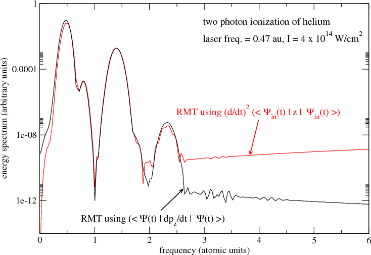
In Fig. 2 we show the results of an RMT calculation of the energy spectrum of scattered light. The energy spectrum is proportional to |E_z(ω)|², where ω is the frequency of the scattered light, and E_z(ω) is the Fourier transform of the time-evolving electric field of the scattered light in the z direction, E_z(t). The energy spectrum gives the total energy scattered in a frequency range. By Parceval’s Theorem, the integration over all frequencies ω of |E_z(ω)|² equals the integration over all time of |E_z(t)|². The latter quantity is proportional to the intensity of scattered light as measured by a detector in the far field, (a great distance from the atom). Intensity of light has the units: joules per second per square meter. Integration of intensity over all time (really over the length of the pulse) would yield the total energy (joules) contained in the z component of the electric field, as measured by a perfect detector (per square meter of the detector). Similarly, integration over a frequency range of |E_z(ω)|² would yield, up to proportionality constant, the energy measured by a frequency sensitive detector in that frequency range. The absolute values of the intensity and of the energy spectrum depend on the systems of units, and the geometry and position of the detector, which are not of interest in the software testing. Units are therefore arbitrary.

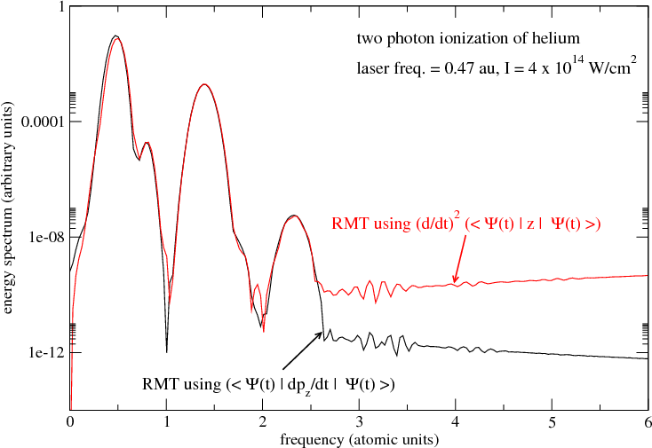
Figure 2 compares the energy spectrum as calculated by acceleration expectation values (Eq. 5) with the spectrum obtained by dipole expectation values. The expectation values are obtained by using only the RMT inner region (B-Spline) wavefunction. For comparison, Fig. 3 shows the calculation repeated with the outer region (finite-difference) RMT wavefunction added in. The use of the full wavefunction in Fig. 3 results in a small but detectable improvement in the agreement between the two methods of calculating the spectrum. The dipole method now agrees well with the acceleration calculation at the 3rd peak (5th harmonic), and gives a background (the high frequency limit of the spectrum) which is smaller than the corresponding background in Fig. 2.

3 Work Package 2. Implementation of HHG code in HELIUM

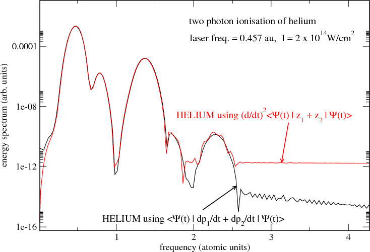
In this section we test the upgraded HELIUM code on a similar case as that used to test the new RMT code in the previous section, namely a comparison of the high harmonic spectrum derived from acceleration expectation values with that derived from dipole expectation values. Again, the TDSE for helium in a short high frequency (0.457 au) laser pulse is numerically integrated and the dipole and acceleration expectation values are tabulated over the duration of the pulse. In HELIUM there is only one region, so no additional MPI communication software was required, but the integration is over two electrons (6 dimensional) instead of one. The dipole expectation values are < ψ(r₁,r₂,t)|z₁ + z₂|ψ(r₁,r₂,t) > , and the acceleration expectation values < ψ(r₁,r₂,t)|dp₁∕dt + dp₂∕dt|ψ(r₁,r₂,t) >.

Figure 4 shows the results of a HELIUM calculation the energy spectrum of scattered light. The energy spectrum is proportional to |E_z(ω)|², the Fourier transform (modulus squared) of the electric field of the scattered light, E_z(t). The meanings of these quantities are discussed in more detail in the previous section. Again we find that if dipole expectation values are used to calculate the energy spectrum then the high frequency part of the spectrum is less accurate than the acceleration calculation.

Figure 4: Energy spectrum of radiation scattered by a helium atom irradiated by a 2 × 1014W∕cm2 laser pulse linearly polarized in the z direction. The spectrum is proportional to the square modulus of the Fourier transform of the time-varying expectation value of the sum of the accelerations of the 2 helium electrons (black curve): < ψ(t)||ψ(t) >, where z = z1 + z2, and zi is the z coordinate of the i-th electron. The same quantity is also calculated from the 2nd time derivative of < ψ(t)|z|ψ(t) > (red curve). Ionisation is driven by an 8 field period laser pulse ramped on over 4 field periods by a sinusoidal ramp, and ramped off identically over 4 field periods.

4 Work Package 3. Tuning the RMT HHG calculation for numerical accuracy

In this section we present a series of comparisons between the predictions of RMT and those of HELIUM over a range of UV laser frequencies (0.1168 au to 0.94 au). Good agreement is observed between the two methods, confirming that the RMT integration parameters have been properly tuned to produce numerical integrations comparable in quality to those of HELIUM. The success of these tests does much to increase confidence in the correctness of the two highly dissimilar numerical integrations.

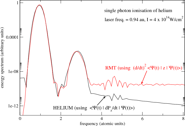
Figure 5 shows the results of the two numerical integrations at the highest laser frequency investigated, 0.94 au. In this case both RMT and HELIUM are used to calculate the energy spectrum. The RMT calculation is based on dipole expectation values, the HELIUM on acceleration expectation values. The results are typical of those presented in the previous sections. The acceleration based calculations have the lower backgrounds (and evidently lower errors) at the higher frequencies. Qualitative agreement is observed over a range of 9 orders of magnitude.

Figure 5: Energy spectrum of radiation scattered by a helium atom irradiated by a 4 × 1014W∕cm2 laser pulse linearly polarized in the z direction. The spectrum is proportional to the square modulus of the Fourier transform of the time-varying expectation value of the sum of the accelerations of the 2 helium electrons (black curve): < ψ(t)||ψ(t) >, where the acceleration = dPz∕dt, z = z1+z2, and zi is the z coordinate of the i-th electron. The RMT curve is obtained from the 2nd time derivative of < ψ(t)|z|ψ(t) > (red curve). Ionisation is driven by an 8 field period laser pulse ramped on over 4 field periods by a sinusoidal ramp, and ramped off identically over 4 field periods.

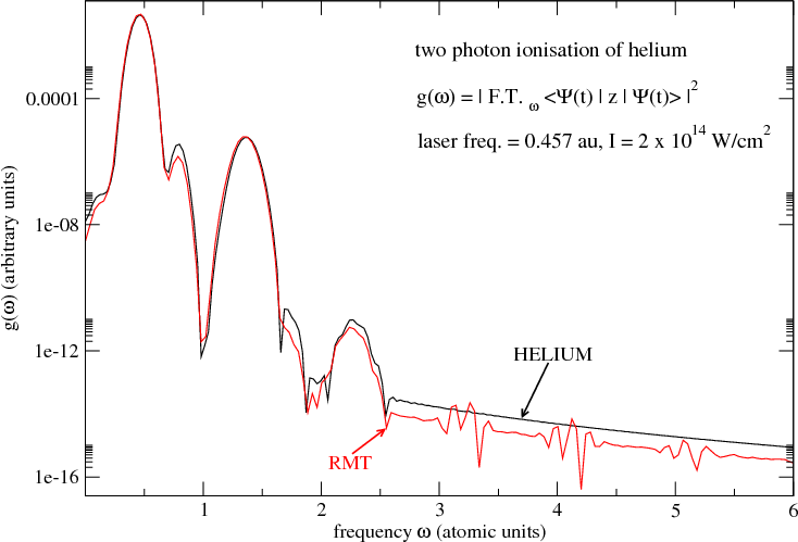
Figure 6 displays the results of a more direct comparison of the RMT and HELIUM integrations than the results shown in Fig. 5. In Fig. 6 the laser pulse characteristic are the same as those of Fig. 4, but in the case of Fig. 6 only the Fourier transforms of the dipole expectation values are shown. To obtain the good agreement between RMT and HELIUM observed in Fig. 6 the RMT inner region required a much larger basis set of splines than originally anticipated. The RMT integration used 48 splines in a 20 atomic unit inner region, which effectively supports inner region excitations as high as 300 au in energy. The RMT outer region used a spatial grid point spacing of 0.166 atomic units, and a maximum angular momentum (single-electron) of 6 ℏ. The RMT outer region Hamiltonian was modelled with 9-point finite-difference, correct to 8th order in the grid point spacing. Grid point spacings larger than 0.166 au caused stability problems in the RMT integration. The stability problem became apparent when the basis set of 48 rather than 30 splines was used. The special feature of the larger basis set is the existence of a high energy, high curvature spline that lies adjacent the outer region boundary. The outer region finite-difference operators sample the inner near this boundary, and therefore sample wavefunctions modelled by this high curvature spline. It is likely that the stability problems occur when the finite-differencing is too coarse to accurately sample the rapid spatial variation supported by the high energy boundary spline.

The HELIUM integration used a spatial grid point spacing of 0.29 au, (which is the standard setting in HELIUM). The integration was repeated with a grid point spacing of 0.20 au with no significant change in results. The HELIUM integration used the same maximum angular momentum as the RMT outer region.

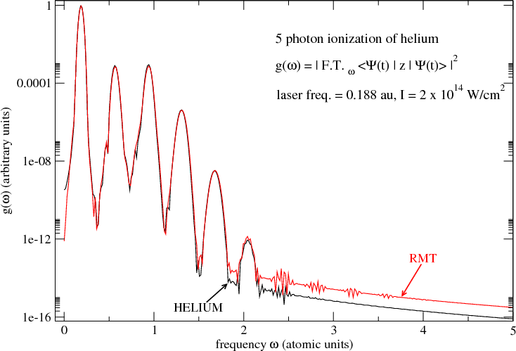
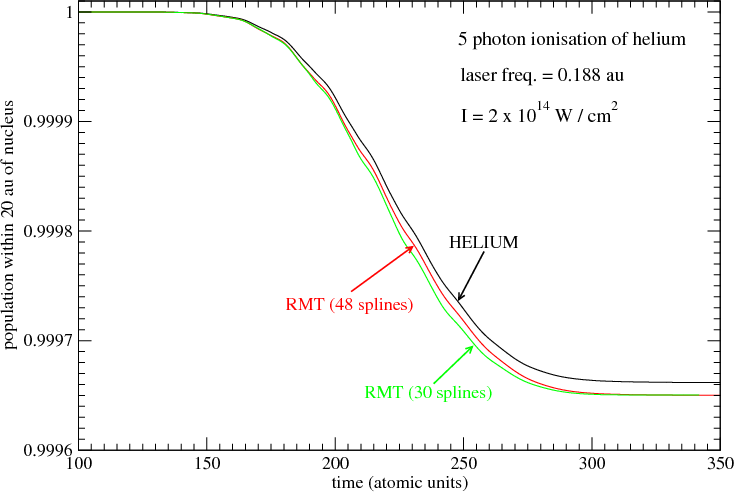
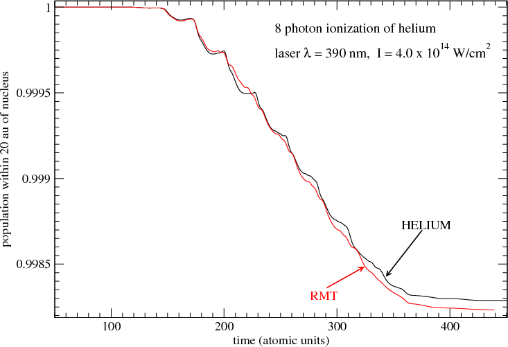
Figure 7 compares the HELIUM and RMT predictions of g(ω). In this case (5 photon ionisation) both the HELIUM and RMT integrations use basis sets with peak angular momentum (single-electron) of 8 ℏ. The RMT integration again used 48 splines in the 20 atomic unit inner region, spatial grid point spacings of 0.166 atomic units in the outer region. Figure 8 compares the single-electron ionisation rates predicted by the HELIUM with those of the RMT integration. As in the case of two-photon ionisation (Fig. 6), the integration did not converge until at least 48 basis splines were used in the inner region. A 64 spline inner region basis gave the same results as 48 splines. The 64 spline basis allowed excitations as high as 600 au in energy, twice that of the 48 spline basis. The HELIUM and RMT prediction of ionisation yield at the end of the pulse differ by under 5%, which is roughly the expected uncertainty in both of the numerical integrations.

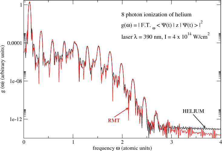
We conclude with the 390 nm results, the longest wavelength used in this series of tests. 390 nm is of considerable experimental interest because it is readily obtained from frequency doubled Ti-Sapphire 780 nm lasers. In Fig. 9 we see the first indication of a broad plateau of harmonic peaks, a phenomenon that makes HHG of such interest and potential value in experimental study. Again there is striking agreement between the two methods over a range of 12 orders of magnitude. A small but interesting discrepancy between the results is evident in the 5th and 7th harmonics. Recent calculations of these spectra, [21], shed some light on this discrepancy. All of the results presented here use the simplest RMT model of helium, called a 1-state model, in which the final-state residual ion (He⁺) is restricted to its 1s ground state. The more recent calculations, [21], exploit a more sophisticated model called the 3-state model, in which the final-state residual He⁺ ion can be not just in its 1s ground state, but also in the two most likely excited states. The 3-state model calculation is more computationally laborious, perhaps by an order of magnitude, but the 3-state results exactly match those of HELIUM in the 5th and 7th harmonics, identifying the likely source of the discrepancy. It is interesting that as RMT approaches HELIUM in the quality of its results, it also approaches HELIUM in computational overhead. The Fig. 9 HELIUM result required about 6 hours on 4000 cores of HECToR. The 1-state RMT integration was at least an order of magnitude faster than HELIUM, but not the 3-state calculation. The great advantage of RMT is that it can be applied to more complex many-electron atoms like neon and argon, which are in common use by experimentalists.

Acknowledgements: This project was funded under the HECToR Distributed Computational Science and Engineering (CSE) Service operated by NAG Ltd. HECToR - A Research Councils UK High End Computing Service - is the UK’s national supercomputing service, managed by EPSRC on behalf of the participating Research Councils. Its mission is to support capability science and engineering in UK academia. The HECToR supercomputers are managed by UoE HPCx Ltd and the CSE Support Service is provided by NAG Ltd.

References