Abstract

The RMT method (R-Matrix with time-dependence) is a new ab initio method for solving the time-dependent Schrödinger Equation (TDSE) for multi-electron atomic and molecular systems in intense short laser pulses. Although several other time-dependent R-Matrix methods have been introduced in recent years [1, 2, 3, 4, 5, 6], RMT demonstrates orders-of-magnitude improvements in efficiency, primarily because it employs finite-difference (FD) techniques to model the few-electron wavefunction far from the atomic core. RMT merges the Outer Region FD model with a classic B-Spline R-Matrix basis set for the multi-electron Inner Region [7]. The difficult problem of merging a basis set model with a spatially adjacent FD model, while maintaining the unitarity of the time-propagator, has been a long-standing barrier to progress in this field. RMT is based on the solution first published in 2008 by Nikolopoulos, Parker and Taylor [8]. We have now shown that this method is both computationally stable and highly efficient.

An implementation of RMT has now been completed and parallelized on workstations, mid-sized parallel machines and on HECToR. Success was due to the use of a mature R-matrix parallel code for the Inner Region, and the use of the HELIUM finite-difference code for the Outer Region [9, 10]. HELIUM [11, 12] has been in heavy use on massively parallel machines since the arrival of the original Cray T3D over 15 years ago. It allows accurate full-dimensionality solutions of the time-dependent Schrödinger equation for two-electron atoms or ions in intense fields. It has demonstrated high parallel efficiency on massively parallel processors, with production runs on over 16,000 cores of HECToR, and successful tests on over 60,000 cores of Jaguar, HECToR’s sister computer at Oak Ridge. It has performed well in similarly rigorous testing on the IBM Blue Gene architecture. It is regularly used on single processor machines, 8-core workstations, clusters of workstations, and large Beowulf-type workstation clusters.

HELIUM was designed to generate high-integrity solutions of the full TDSE for laser-driven 2-electron atoms. Experience with HELIUM demonstrates that a very basic requirement for high accuracy results is the use of large integration volumes - in other words the use of Outer Regions of 1000’s of Bohr radii in extent. Attempts to truncate the integration to boxes of much smaller radii invariably produced unacceptable and difficult to detect integration errors. Of equal importance is the fact that the basic problem of calculating the energy spectra of ejected electrons is intractable without a high-accuracy treatment of the wavefunction for these electrons as they travel far from the nuclear core. For this reason, the HELIUM finite-difference approach and HELIUM algorithmic methods for the propagator are considered mandatory if the RMT method is to generate solutions of the TDSE comparable in accuracy to those obtained by HELIUM for purely two-electron systems.

Over the last 5 years, remarkable advances in laser technology have enabled experimental study of matter-laser interactions with unprecedented time-resolution. Experiments can now be performed using few-cycle pulses of high-intensity Ti:Sapphire laser light at  800 nm wavelengths, and at Vacuum-Ultraviolet wavelengths (VUV) with pulses as short as  250 attoseconds. The creation of attosecond pulses in particular has opened up a new frontier in the study of ultra-fast electronic processes. Recent landmark attosecond spectroscopic measurements in a solid [13] have demonstrated that ultra-fast techniques can probe solid state processes occurring at the theoretical ultimate speed limit for electronics. Attosecond pulses have recently enabled the real-time observation of electron tunnelling in atoms [14] and Auger decay of inner-shell electrons [15]. Attosecond pulses have also enabled stroboscopic study of single ionization events in argon [16].

Interactions that occur over a few cycles of the laser pulse, either due to the extreme intensity of the pulse, or due to the short duration of the pulse, cannot be reliably modelled with traditional time-independent methods. If theory is to play a meaningful role, and especially a predictive one, in such circumstances, then sophisticated methods of calculation are required which will be capable of accurately describing both the multi-electron atomic structure and the time-dependent multi-electron response to the light field.

R-matrix methods successfully model multi-electron atom-laser interactions, and molecule-laser interactions, but only in the time-independent limit. HELIUM successfully models time-dependent atom-laser interactions, but is limited to 2-electron atoms. RMT removes both of these limitations. Through the use of the R-matrix method it allows a truly multi-electron dynamical description of the Inner Region near the nucleus where all the electrons of the system can be found. This is important because in the high-frequency limit, (VUV and XUV (extreme ultraviolet)), inner-shell excitations can be expected to influence or dominate the interaction. The use of finite-difference methods derived from HELIUM provides a high accuracy description of the Outer Region of space which, although very large in comparison to the Inner Region, is accessed by at most two electrons in double ionization processes (just a single electron for single ionization). Of equal importance to the success of RMT is the high efficiency and scalability on parallel computers of the HELIUM approach.

In summary, the goal of RMT has been to enable theoretical analysis of recent experimental advances with a degree of reliability that would be impossible by competing methods. These include time-resolved studies of ionization events in attosecond time-scales, studies of time-delays between the ejection of electrons in double-ionization, inner shell excitations and decays in complex atoms, intense-field atom-laser interactions in the XUV limit using the new free-electron x-ray lasers, and harmonic generation in atoms and molecules.

Contents

1 Objectives and Outcomes

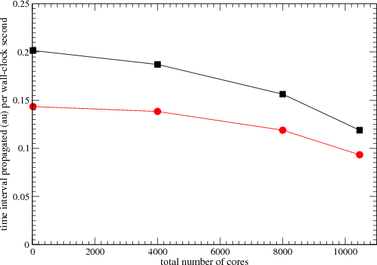
In section 2 we discuss the goals and outcomes of Work Package 1. The objective of Work Package 1 was to develop and test a series of optimizations for efficient load balancing of the RMT Inner Region (I.R.) with RMT Outer Region (O.R.). Figure 1 and related text discuss the scaling laws and benchmarks used to choose optimal parameters for the balanced execution on jobs in the 100-10,000 core range. Tests were performed on configurations with 100-1000 I.R. cores, and 100-10,000 O.R. cores.

Figures 2 and 3 and related text discuss an optimization that modified the order of communications between the I.R. and the O.R.. We call this the Red-Black optimization, and demonstrate a case in which it gives us a factor 1.7 increase in integration speed, in the limit of greater than 500 I.R. cores. We remark that the result of this optimization is fortuitous: with the addition of 340 cores to the I.R., it is for example possible to increase the speed of an 8,000 core program by 70%.

We describe 2 additional successful optimizations: 1) moving computation from the O.R. to the I.R (thereby reducing the information exchanged between the regions each time-step), and 2) the assignment of a single dedicated core to inter-region communication. Together these optimizations gave a significant speed-up, as shown in Figure 1. We investigated upgrading the present MPI design with potentially faster MPI collectives, but the MPI collectives were rejected due to incompatibilities with the complicated MPI methods used in the Red-Black scheme.

In section 3 we discuss the goals and outcomes of Work Package 2. The objective of Work Package 2 was to implement an algorithmic enhancement to the propagator in order to improve efficiency in the limit of small spatial grid-point spacings. The original proposal involved exponentiating an approximation of the Hamiltonian, but the computational overhead of this approach exceeded the improved efficiency. Instead we developed a method based on least-squares finite-difference operators that successfully produced the desired improvement in integration speed. In section 3 we show that the least-squares finite-difference methods retain the accuracy of the original 5-point finite-difference rules, but improve stability by suppressing the highest frequency modes on the finite-difference grid, thereby allowing larger integration step-sizes and integration speed. We present the results of an integration in which the least-squares rules increase integration speed by a factor of 1.8 over that of the standard 5-point finite-difference rule, exceeding the original goal of a 50% improvement in speed.

2 Work Package 1. Optimization of the MPI implementation of RMT for HECToR and likely successors

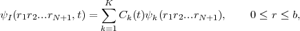
We begin with a brief account of how HELIUM methods addressing the few-electron Outer Region are combined with R-matrix basis set methods handling the multi-electron Inner Region. We write in the Inner Region I where all electrons can be found:

(1)

where ψ_k(r₁r₂...r_N+1),k = 1,K form a field-free, time-independent R-matrix basis for the (N + 1) electrons within the Inner Region with outer boundary at r = b. The construction of the ψ_k is the responsibility of long-existing atomic R-matrix time-independent codes. The time evolution of the Inner Region time-dependent wavefunction is entirely contained in the coefficients C_k(t) whose time evolution is determined by the TDSE. However in writing the TDSE we must take care that the Hamiltonian and dipole operators which act on ψ_I(r₁r₂...r_N+1,t) are Hermitian over Inner Region I (where ψ_I(r,t) is only defined). The Hermitian Inner Region Hamiltonian is given by H_I = H₀ + _h and the dipole operator by D_I = D + _d, where _h and _d are Bloch surface terms, only non-zero at r = b. In these circumstances the TDSE over Inner Region I is written:

(2)

where 0 ≤ r ≤ b.

This equation is a key one to the method. The second term on the right hand side compensates for the Bloch terms introduced to make H_I and D_I Hermitian. Note that it makes a contribution only at r = b and brings into play there ψ(r,t) a one-electron wavefunction form which we define from just within the Inner Region outwards. This term is central to any time propagation scheme in Inner Region I because it connects the wavefunction form ψ_I(r₁r₂...r_N+1,t) specific to that region with a wavefunction form that at r = b represents a single electron and which in calculations is obtained from Outer Region II.

The Outer Region II is spanned by a finite-difference (FD) grid so that the one-electron wavefunction there is written

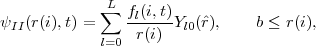(3)

with i = i_b,..,I and r(i_b) = b. In this form, for simplicity of presentation, we have allowed for only one residual ion state of the system. The form the TDSE takes in this Outer Region is then

(4)

This, the second key equation to the method, is the normal form of the TDSE over a FD grid except for the terms multiplying δ_iib and δ_iib+1. Note that these terms require quantities (the Bs) to be evaluated at grid points i_b - 1 and i_b - 2 i.e. at points on the inner side of the boundary at r = b. This reflects the use of 5-point difference operators on the FD grid.

We emphasize how Eqs. (2) and (4) are actually used by sketching the computational procedure in propagating the full wavefunction through one time-step from t to t + τ. We first consider the Outer Region TDSE, Eq. (4). This is handled by the explicit Arnoldi time-propagator method [11] as in HELIUM and brings into play Inner Region information through the B_0l(i_b - 1,t), B_0l(i_b - 2,t) and B_1l(i_b - 1,t) terms all known from time t. Having thus determined all the f_l(i,t + τ) for i = i_b,..,I we proceed to the Inner Region. What we need to determine here are the coefficients C_k(t + τ) and again these are determined by the explicit Arnoldi time-propagator using knowledge of the Outer Region f_l(i,t + τ) to determine the spatial derivative terms at r = b brought in by the non-zero Bloch operator terms there.
Attempts to create efficient time-dependent R-matrix integrations for such large volumes have made slow progress, largely because successful integration of the relevant high-dimensional partial differential equations is so computationally demanding that it requires the benefit of parallelization over tens of thousands of cores, which is not straightforward in pure R-Matrix formalisms.

To enable the RMT code to run efficiently on HECToR, this work package focused on improving load balancing among the cores, and improving the efficiency of communications between cores the Inner Region (I.R.) cores and Outer Region (O.R.).

Load balancing concerns minimizing the idle time of HECToR cores during the run. As the computational algorithms implemented by cores in the Inner and Outer Regions are vastly different, the computational effort it takes to propagate the wavefunction forward one step in time will be different in the two regions. Therefore for the RMT code to run efficiently on HECToR it is imperative that an understanding of the relative computational effort between Inner and Outer Regions is built up through experience of running the code for different conditions. In the Inner Region (I.R.), the propagation forward in time involves a matrix-vector multiplication.

The matrix has a block tri-diagonal form; the blocks consist of matrix elements coupling two values of total angular momentum. The I.R. is parallelized over these block structures, so that for total angular momentum ranging from zero up to some maximum value, the minimum number of cores used will be that value plus one. Each core then handles a sub-section of the matrix-vector multiplication.

In the Outer Region (O.R.) the computation is a domain decomposition over the grid points. Each core handles a segment of the wavefunction, and stores it in an array of dimension N_grid × N_channels where N_grid is the number of grid points and N_channels is the number of channels. The number of channels is dependent on the value of total angular momentum and the number of residual target states retained in the calculation.

Given the value of total angular momentum and the number of residual target states there should be some optimal value of grid points per core that will best balance the computation performed by the cores in the two regions. The desired values of the total angular momentum and the number of residual target states are dependent on the scientific problem at hand. To give an indication of the types of problems we anticipate studying with RMT, consider the neon atom. Neon has a multitude of residual ion target states that are very close together in energy: retaining 8 (21) of these and allowing angular momentum values up to 24 (30) gives around 500 (1500) channels and an I.R. Hamiltonian of dimension 25000 (120,000). To propagate the wavefunction accurately over the course of an intense 10 cycle infra-red laser field would require a radial grid extending as far as 20,000-35,000 Bohr radii. Sometimes it is necessary to resolve resonance structures: in these extreme cases, integration over many (greater than 100) field periods becomes necessary, and consequently the radial grid must extend further by one to two orders of magnitude. We estimate that these types of calculations would require 100-1000 cores to handle the I.R. and 200-10,000 cores to handle the O.R.

Load balancing on 200-10,000 cores

We turn now the problem of choosing optimal parameters for balanced computation in the practical limits RMT was designed for. Of special interest is the case in which the outer region (O.R.) encompasses core counts as high as 10,000. This is expected to be a typical core count in studies of intense-field harmonic generation studies, one of the original motivations for the creation of the RMT method.

In this section we test O.R. core counts in the 100-10,000 range, with inner region core counts fixed to 100 cores. In the following section on the Red-Black optimization, we explore varying the I.R. core counts up to 1000 cores.

We start with the general problem of balancing the workload between the inner region (I.R.) and outer region for arbitrary configuration of the R-Matrix inner-region. If the O.R. cores complete their computation too quickly, then they sit idle, waiting for the I.R. to complete. If the O.R. cores have too much work to do per time-step, then the I.R. cores sit idle, waiting for the O.R. to complete. Notice that if the O.R. cores outnumber the I.R. cores by 100 to 1, (a not uncommon case), then I.R. idleness is not very expensive computationally - preventing O.R. core idleness in this limit is the top priority for efficiency.

Parameters defining the R-Matrix I.R. are for the most part constrained to certain values by the physics of the problem. The only easily adjustable parameter is the outer region parameter governing the number of grid points per core: N_grid. It is straightforward to calculate a good estimate of N_grid based on knowledge of the run-time scaling of the I.R. and O.R. as a function of several program parameters. To first approximation, the run-time overhead per time step of the inner region scales as

   runtime_per_step = c_innerN_block²∕N_CPB

where c_inner is a proportionality constant, N_block is the dimension of the matrix block making up the tridiagonal I.R. Hamiltonian block matrix, and N_CPB is the number of I.R. cores allocated per block. Constants accounting for communications overhead can be neglected here. Run-time overhead per time step of the outer region scales as

   runtime_per_step = c_outerN_gridN_channels,

where c_outer is a proportionality constant, N_grid is number of radial grid points per core, and N_channels is the number of channels. Equating the two quantities so that the I.R. and O.R. complete each step in comparable time duration gives us the desired initial estimate for N_grid:

   N_grid = (c_outer∕c_inner)N_block²N_channelsN_CPB.

The ratio c_outer∕c_inner is calculated by repeated trials of the RMT program. If the ratio c_outer∕c_inner is independent of parameters like N_channels etc., then a knowledge of the ratio determines N_grid for all parameter choices. Not surprisingly, the ratio c_outer∕c_inner does not turn out to be a true constant, but varies somewhat with changes in problem parameters, and more substantially with changes in hardware. On HECToR, 1/15 is typical value for c_outer∕c_inner. Figure 1 shows some RMT timings with N_channels = 101,N_block = 673,N_CPB = 5. In this case the optimal N_grid was about 60, and c_outer∕c_inner = 1/15. In another set of benchmarks (not shown) N_block = 430, significantly decreasing the size of the arrays on the I.R. cores, (which improved the efficiency of the I.R. calculation through faster memory access) so that the speed-up was somewhat greater than would be expected from linear scaling in the quantity N_block². The optimal value for the ratio c_outer∕c_inner was in this case about 1/12, due to the smaller c_inner. Figure 1 demonstrates the degraded performance of RMT from MPI communications overhead as core counts approach 10,000.

Optimizing I.R./O.R. computation order: the red-black optimization

The RMT propagator is such that the wavefunction must be known in both regions at the start of any given time step, i.e. effectively both regions synchronize at the start and at the end of each time step. The computation amounts to calculating the Hamiltonian times the wavefunction. The I.R. can do its part independently of the O.R., but the O.R needs some wavefunction information from the I.R. to begin calculation. The first step then is for the I.R. to send wavefunction information to the O.R.. The O.R. cores are idle until they receive this data. When reception is complete, the O.R. begins calculation of H Ψ_II and the I.R. cores become idle. The O.R. completes its first order propagation and sends information to the I.R.. At this stage the I.R. can commence its first order propagation and the O.R. can commence its second order propagation in parallel with the I.R., after which it sends more information to the I.R.. The higher the order of the propagator, the higher percentage of this computation can be done in parallel (i.e., the more the I.R. can work independently of the O.R.). This process repeats up to the maximum order of the Arnoldi propagator. (Arnoldi propagators are used in both regions and the maximum propagation order is a parameter in the code.) Finally the I.R. can complete its maximum order propagation, and the two regions can again synchronize.

We find that we can increase the degree to which the Inner and Outer regions work independently of each other by dividing the I.R. into two independent sets of cores - which we call red and black cores. This optimization works by allowing the red I.R. cores and the black I.R. cores to independently receive information from the O.R. In certain limits this independence improves I.R. parallelism by allowing one set of cores to begin computation instead of sitting idle awaiting the other set to synchronize with the O.R. As we show below, the availability if this option improves the program’s ability to exploit large numbers of cores as well as the overall efficiency of the integration.

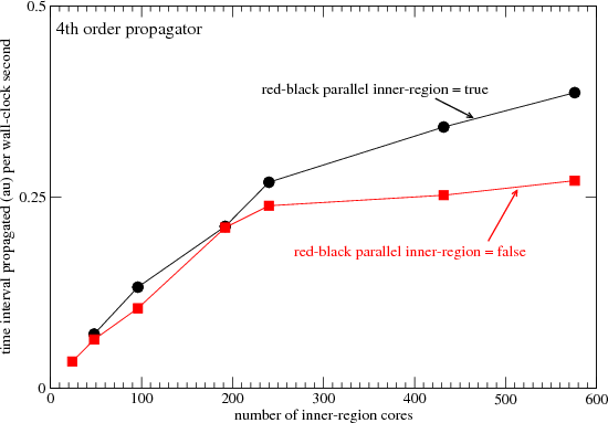
In Figures 2 and 3 the outer region overhead (per core) has been reduced to its ultimate minimum by using just 32 grid points per core. The Hamiltonian assumes a maximum angular momentum L_max = 23, so the inner region Hamiltonian is a 24 x 24 block tridiagonal matrix. The number of cores over which the inner region is parallelized must therefore be a multiple of 24. If the red-black optimization is enabled, then the number of inner region cores must be a multiple of 48.

Figures 2 and 3 plot the speed at which the RMT code can integrate the equations of motion. We see in Figure 2 that adding additional cores to the inner-region results in a near linear speed-up up to about 240 I.R. cores. Above 240 I.R. cores, the improvement in speed is negligible for the case in which the red-black decomposition is disabled, but continues linearly (with a smaller proportionality constant) in the case in which red-black decomposition is enabled. At about 580 cores, the integration with the red-black optimization enabled is a factor 1.45 times faster than that of the disabled case. So the addition of 340 I.R. cores above the 240 core threshold (more than doubling the number of inner region cores) yields an improvement of about 45 percent in speed. This may at first glance seem disappointing, but it is both desirable and beneficial in the RMT code. In practice the outer region will run on 1000’s or tens of 1000’s of cores. In the example in Figures 2 and 3, the total number of cores (Inner + Outer) is 8192. If the outer region is using say 8192 cores, then the addition of 340 I.R. cores is a highly inexpensive way to improve the run-time efficiency of the entire program by 45 percent.

Figures 2 and 3 show only up to about 600 I.R. cores. The tests were performed up to 1000 I.R. cores, but little or no improvement was observed above 600 cores. The matrix computations that were parallelized by these 600 cores were performed on matrices that were 552 x 552 in dimension. In some RMT problems, matrices up to 30,000 x 30,000 in size have been used, and it is expected that in this case the addition of more than 600 cores will provide additional speedup.

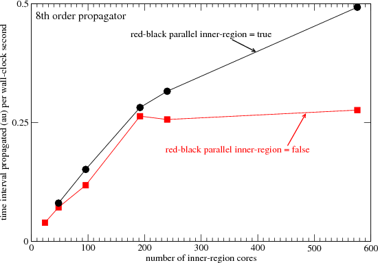
The results plotted in Figure 3 demonstrate that we can obtain even better parallelism by using a higher order (8th order) propagator. In this case, with the red-black optimization enabled, speed is factor 1.7 times greater than that of the disabled case. This is another fortunate result, because the Arnoldi propagator improves in overall efficiency with order. More precisely, doubling the order of the Arnoldi propagator usually doubles the run-time, but allows time-steps to more than double for a net gain in integration speed. In practice, the highest order possible within the constraints of available memory is used. Order 12 to 16 is standard.

Optimizing communications between the Inner and Outer Regions

Each time step the Hamiltonian-wavefunction product is calculated numerous times, and each time it is calculated information must be exchanged between the I.R. and the O.R. cores. Several approaches to improving the efficiency of this process were investigated.

The second term on the right hand side of Eq. (2) must be calculated in the O.R. and then sent to the I.R.. As outlined above, each I.R. core is responsible for a subsection of the matrix-vector multiplication, and therefore this O.R. data is needed on all I.R. cores. As a possible optimization of this process we considered a new communications design using MPI’s single-core to many-core collectives. These optimization attempts failed because they were incompatible with the complicated parallelization and communications scheme arising from the new Red-Black optimization described above.

Another impediment to efficient inter-region communication was a large penalty that arose from the O.R. computation of surface amplitudes for use by the I.R. Each time step a (potentially large) vector is repeatedly calculated in the O.R. via a projection of each channel wavefunction’s radial derivative onto known time-independent surface amplitudes, and sent to the I.R.. This computation was moved from the O.R. to the I.R. based on the observation that in the limit of optimal load balancing, it is the I.R. that will be privileged with greater idleness, hence will have the spare CPU cycles to devote to the calculation.

Originally we also proposed to reduce the size of the data packets transferred between the inner and outer regions, but instead the modifications described in work package 2 resulted in a large increase in the size of these data packets. Fortunately, this additional burden was removed by the following optimization: a single O.R. core was dedicated to the data transfer, and any excess time remaining (compared to the run-time per step of other O.R. cores) was applied to propagating the O.R. Hamiltonian over a reduced workload, so that it was exactly synchronized with the remaining O.R.cores. Figure 1 shows the improvement (squares) in the speed of RMT with this optimization on 100 to 10,000 O.R. cores.

3 Work Package 2. Algorithmic enhancement of the time propagator

In certain limits, (for example in the limit of high nuclear charge Z) the finite-difference Outer Region integration becomes excessively inefficient in comparison to the Inner Region time propagation. A straightforward enhancement to the present propagation algorithm, yields significant improvements in efficiency, and can restore balance between the Inner and Outer Regions in these limits. The difficulties are particularly acute when highly-stripped ions are modelled, because of the need to make the grid point spacing small in these cases. In a typical problem, using HELIUM to model a 2-electron atom with Z = 2, a choice of δr = 0.25 au proves satisfactory. By contrast, for He-like neon (a highly stripped ion with Z = 10, and a charge of 8 e) we find that a δr = 0.025 au is a more satisfactory choice.

Unfortunately, the Outer Region (O.R.) requires integration time-steps δt that scale as 1∕δr². In other words, if we decrease δr by a factor of 10 from δr = 0.25 au to δr = 0.025 au, then we must decrease δt by a factor of 10000, and the program runs (at least) 10000 slower. The difficulty arises because the highest energy eigenvalues of the finite-difference Hamiltonian are of the order E = ℏ²k²∕2m where k_max² = 10∕δr². These high energy eigenstates can be thought of to first approximation as the most energetic plane-waves that the grid can support. They are unphysical excitations, and in general should contain no population. They tend to be one, two or more orders of magnitude greater in energy that the physical plane-waves excited by the laser pulse, (the plane-waves that represent ionizing electrons). For example, at δr = 0.25 au, the physical excitations are rarely greater than 10 au in energy. But at δr = 0.25 au, the highest energy eigenvalues E on the grid are observed to be of the order 100 au, (using typical integration parameters). At δr = 0.025 au, the corresponding energies are of the order E = 10000 au. Unfortunately, the propagator must successfully integrate the equations of motion as though these high-energy unphysical modes contain population. Otherwise, spurious population accumulates in these modes through integration error - the integration becomes unstable and fails catastrophically. In the explicit propagators used by HELIUM and RMT, stability is regained as δt, the integration step size, is decreased to something of the order of the period of the highest energy plane-wave supported by the finite-difference grid, which, as explained above scales as 1∕δr².

The finite-difference portion of the RMT code is the outer region (O.R.) portion of the integration. The O.R. is very typically a distance 20 au or more from the atomic core. At this distance the atomic Coulomb potentials arising from the attractive forces between the ejected (ionizing) electron and the nuclear core, and the repulsive forces between the ejected electron and the remaining electrons are relatively weak. The eigenvalues of the finite-difference Hamiltonian are dominated by the Kinetic Energy operator K. The eigenspectrum of the Kinetic Energy operator K is in turn dominated by that of the 2nd derivative operator. (The centripetal repulsion term falls off as the inverse square of r, and makes a negligible contribution to the spectrum.) The electric field also influences the eigenspectrum. At typical field intensities it may shift the field-free peak eigenvalues by something of the order 5-20 percent, but rarely more. Except in the most extreme circumstances, the eigenspectrum of the outer region Hamiltonian is to good first approximation that of the 2nd derivative operator appearing in K (multiplied by -0.5∕δr²).

We would expect then, that in the limit of small δr the integration step size δt is governed by the 1∕δr² dependence of the 2nd derivative finite-difference operator of the Kinetic Energy operator K. This is in fact what we observe in the normal operation of the RMT code. Since both the inner region and outer region use the same step size δt, the behavior of the eigenspectrum of K has a profound effect on the run-time efficiency of the RMT code. Developing methods of mitigating the effect of the high eigenvalues of K has been the goal of workpackage 2. The originally proposed method involved exponentiating K, or of an approximate K, independently of the remaining parts of the Hamiltonian. The computational overhead of this method of this method proved to be greater than the cost savings from the larger step size δt, so this method was abandoned. Instead we developed a method of reducing the peak eigenvectors of K by using least-squares operators. The new technique successfully reduces the peak eigenvalues of K by up to a factor of 4, and does so at very little additional computational cost. In fact in most cases the additional computation is undetectable in the run-time of the RMT.

We turn now to a demonstration of the new technique, and discuss a case in which δt can be increased by a factor of 1.8 over that of the original code. The integration proceeds with same accuracy and stability as the original code, but 80 percent faster than the best speed possible by the original code. The new technique appears to be a nearly ideal solution to the problem.

We begin by outlining the methods used to generate the least-squares finite-difference operators.

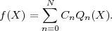
If function f(X) is written as an Nth order polynomial, or equivalently as a linear combination of N+1 orthogonal polynomials Q_j(X) of orders j = 0 to N, then finite-difference differentiation and integration rules can be derived by taking derivatives and integrals of the polynomial representation of f(X). The use of orthogonal polynomials, as described in the following, makes it easy to create a least-squares representation of f(X) and of finite-difference differentiation and integration matrix operators.

Let f(X) be a linear combination of orthogonal polynomials Q_n(X):

(5)

Here the C_n are determined by projecting both sides of the above equation onto polynomial Q_n(X). By the orthogonality of Q, (i.e. (Q_m,Q_n) = 0 if n≠m), we get

(6)

The inner product (f,Q_m) with respect weights W_j is defined:

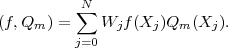(7)

Notice we do not assume that the Q’s have been normalized. Inserting the value of C_n derived above into the polynomial expansion of f(X), and inverting the order of the sums over j and n gives the desired rule:

(8)

The sum over j is over data points X_j. The sum over n is over polynomials Q_n. To interpolate, integrate or differentiate f(X), we use its polynomial representation, given by equation 8 above. For example, differentiation of both sides of the above formula yields a rule for taking the derivatives of f(X).

A sum of N+1 orthogonal polynomials, up to order N, will exactly approximate any tabular function of N+1 points f(X₀),f(X₁),...f(X_N). If the sum is truncated to less than N+1 polynomials, then the result is a least-squares fit to these points. Generally we throw out the high order polys, Q_N,Q_N-1,... because they contain the highest frequency components of f(X), (the components that rapidly oscillate as X varies).

As an example, we now write down the steps used to create a least-squares finite-difference 1st derivative of f(X). Differentiating Equation 8 on both sides of the equality gives:

(9)

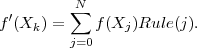
The finite-difference differentiation rule at point X_k is the set of numbers in brackets [], which we call Rule(j):

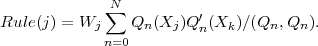(10)

With this definition, equation 9 becomes a finite-difference rule for differentiation at X_k:

(11)

To generate the orthogonal polynomials Q and the derivatives of Q, the Gram-Schmidt recurrence relation is used.

(12)

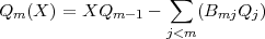(13)

The sum on the RHS was added to make Q_m orthogonal to all previous Q’s. The coefficients B_mj that guarantee orthogonality are:

(14)

where (P₁,P₂) denotes the weighted inner-product defined above. To see this take the inner product of the equation for Q_m with Q_j, assuming j < m, set it equal to zero, and use recursion. The form given above is the one that generalizes to many dimensions. In one dimension the formula simplifies so that only two of the B coefficients are nonzero. We call these coefficients A_m and B_m:

(15)

(16)

(17)

where

(18)

(19)

Differentiating both sides of the above recurrence relations for Q(X) gives the desired recurrence relations for the higher order derivatives of Q(X).

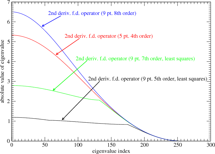
Figure 4 shows the eigen-spectra of two least-squares finite-difference operators along with the eigen-spectra of two non least-squares operators.

The eigenvectors in this example are to good approximation sinusoids. In the limit of infinitely small grid-point spacings, the operator becomes and its eigenvectors approach exp(ikr), with eigenvalues -k²:

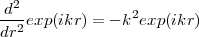(20)

In Figure 4, ”order” refers to the order of the polynomial used to calculate the 2nd derivative. For example, in the case of the 9 point rule, the non least-squares operator is 8th order. In other words, an 8th order polynomial is chosen such that it passes through each of the 9 points. The 9 point rule returns the exact 2nd derivative of this polynomial at the central point. An 8th order polynomial is the lowest order polynomial that can in general pass through any arbitrarily chosen 9 points. The least-squares rules use polynomials of order less than 8. These polynomials do not in general pass through each of the 9 points. For this reason they are less sensitive to numerical noise that accumulates during the numerical integration of functions that can be described as linear combinations of exp(ikr). It is apparent that the least-squares process can dramatically truncate the higher frequency components of the eigen-spectrum without significantly changing the low frequency components.

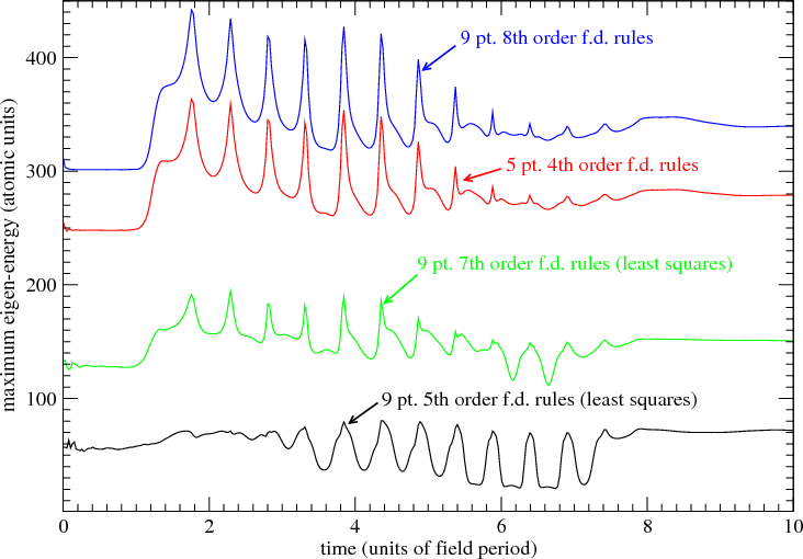
Figure 5 shows the resulting reduction in peak eigenenergies when the least-squares finite-difference operators described above are substituted into the RMT outer region Hamiltonian. The peak eigenvalues shown in Figure 5 are not physical excitation of the atomic system. The highest eigenvalues shown in Fig. 5 are 10 to 100 times larger in energy than the energies of the electrons excited by the laser. They are numerical artifacts of the finite-difference grid. By suppressing them, we can can use larger integration step-sizes δt while maintaining both stability and accuracy. 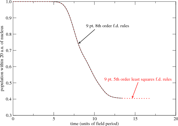Figure 6 demonstrates that the least-squares rules give the same answers as the non least-squares rules.

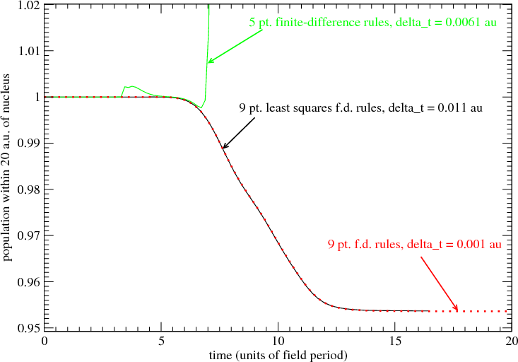
Figure 7 demonstrates that the 9 point least-squares operator enables integration step-sizes significantly larger than step-sizes possible with the non least-squares 5 point rule. The 5 point rule results in a catastrophic integration failure at a rather small δt. The failure is due to instability in the integration that becomes apparent at δt = 0.0061 au. For all larger δt, the instability worsens. The integration using least-squares finite-difference rules (9 point, 5th order, black line) is stable and accurate at δt = 0.011 au. (In these two examples the grid point spacing is δr = 0.05 au.) Results using a smaller grid point spacing δr = 0.001 au, along with the most accurate of the finite-difference rules (red line: 9 point, 8th order) are presented in order to verify the accuracy of the 9 point least-squares rule (black line).

One of the nice features of this approach is the good run-time efficiency of the 9 point rules. On tests of RMT on HECToR, the 9 point rules were nearly as fast as the 5 point rules. It was in fact difficult to detect a difference. This is evidently due to the fact that much of the overhead of the finite-difference computation is in the access of the large wavefunction arrays from memory (rather than in the floating point ”*” and ”+”). This memory fetch overhead is the same for the 9 and 5 point rules. And although the 2nd derivative operator is the cause of the unphysically large eigenvalues of the Hamiltonian, it has a small computational cost in comparison to all the other operators in the Hamiltonian. For this reason, the 9 point RMT runs as fast as the 5 point RMT, and we find that the ability to increase δt by a factor 1.8 directly translates into a factor 1.8 increase in integration speed.

Acknowledgements:

This project was funded under the HECToR Distributed Computational Science and Engineering (CSE) Service operated by NAG Ltd. HECToR - A Research Councils UK High End Computing Service - is the UK’s national supercomputing service, managed by EPSRC on behalf of the participating Research Councils. Its mission is to support capability science and engineering in UK academia. The HECToR supercomputers are managed by UoE HPCx Ltd and the CSE Support Service is provided by NAG Ltd.

References