| ∇ .
|
(1) |
Lucian Anton1, Jacek Dziedzic2&3, Chris-Kriton Skylaris2, and Matt Probert4
1Scientic Computing Department, Science and Technology Facilities Council, Daresbury Laboratory WA4 4AD, U.K.
2School of Chemistry, University of Southampton SO17 1BJ, U.K.
3Faculty of Applied Physics and Mathematics, Gdansk University of Technology, Poland.
4Department of Physics, University of York, Heslington, York, YO10 5DD, U.K.
November 3, 2013
The goal of this project was to develop in Fortran 95 a hybrid parallel (MPI+OpenMP) multigrid solver package scalable to at least 1000 cores for typical problems, tuned to the requirements of the ONETEP [1] and CASTEP [2] codes: continuous charge distributions, variable permittivity function, Dirichlet, Neumann, periodic and mixed boundary conditions, linear Poisson equation (PE) and non-linear case as in the Poisson-Boltzmann equation (PBE).
The parallel multigrid solver DL_MG was developed according to the following specifications:
The following subtasks named in the work packages were not finished in the allocated time. Justification is provided below for each outstanding item:
Implicit solvation models provide a computationally affordable way to model solvent, by representing it as a dielectric continuum which surrounds and is polarised by the solute and "reacts" by back-polarising the solute. In first principles electronic structure calculations this is taken into account in the self-consistent process so that the electronic density is deformed accordingly by the presence of the solvent. Furthermore, a number of explicit solvent molecules can be included when necessary (e.g. water molecules forming hydrogen bonds with an exposed protein active site). A large number of solvation modes have been reported in the literature [3]. The equations relevant to the solvent models in this work are the non-homogeneous Poisson equation:
Classical and quantum-based approaches differ in how they describe the
charge density of the system,
![]() (r). The
former express it as a collection of point charges, represented by
Dirac delta functions [7], the latter use continuous charge
densities, typically represented on a Cartesian grid. This is an
important distinction, as it necessitates implementing different
numerical approaches in the solvers in order to tackle the
corresponding difficulties. The multigrid solver described here is
geared towards electronic structure calculations and thus assumes that
all three quantities of interest (permittivity
(r). The
former express it as a collection of point charges, represented by
Dirac delta functions [7], the latter use continuous charge
densities, typically represented on a Cartesian grid. This is an
important distinction, as it necessitates implementing different
numerical approaches in the solvers in order to tackle the
corresponding difficulties. The multigrid solver described here is
geared towards electronic structure calculations and thus assumes that
all three quantities of interest (permittivity
![]() (r), charge density
(r), charge density
![]() (r), and potential
(r), and potential
![]() (r)) are
continuous and are represented on a Cartesian grid.
(r)) are
continuous and are represented on a Cartesian grid.
However, even in electronic structure methods, the ionic cores are internally represented as point pseudocharges and careful treatment is needed to correctly describe them in the context of a multigrid solver. The so-called smeared-ion formalism [8] can be used to replace the point pseudocharges with Gaussian ("smeared"), Coulombic representation of the cores. In this formalism, the total charge density is expressed as
where
RI is the position of core I, ZI is its charge, and
![]() is a chosen smearing width in the order of
1 a0. Appropriate correction terms to energy [8]
and forces [9] are needed to ensure they remain
unchanged. The dielectric permittivity can be treated in
different ways, depending on the problem at hand. In solvation
calculations it is usually set to a solvent bulk value outside of a
suitably defined cavity around the solute and assumes a value close to
unity inside the cavity. Slightly larger values (2 - 5) are
occasionally used to model screening effects within the solute. Two
main approaches are employed to define the shape of the cavity. In the
first one the cavity is constructed as a set of overlapping
atom-centred spheres, whose radii are parametrised. In the second
approach the permittivity is defined as a function of the electronic
density: ε = ε[ρ] (r). This approach, first
proposed by Fattebert and Gygi [10] and later extended
by Scherlis et al. [9] and Dziedzic et
al. [11] and Andreussi et al. [13]
avoids a discontinuity at the cavity boundary, replacing it with a
steep, but continuous change of the permittivity, which follows
naturally from the change in electronic density. This is the approach
used in ONETEP [11] and CASTEP [12].
Calculations in vacuum use a homogeneous permittivity of 1, whereby
equation (1) simplifies to the homogeneous Poisson equation:
is a chosen smearing width in the order of
1 a0. Appropriate correction terms to energy [8]
and forces [9] are needed to ensure they remain
unchanged. The dielectric permittivity can be treated in
different ways, depending on the problem at hand. In solvation
calculations it is usually set to a solvent bulk value outside of a
suitably defined cavity around the solute and assumes a value close to
unity inside the cavity. Slightly larger values (2 - 5) are
occasionally used to model screening effects within the solute. Two
main approaches are employed to define the shape of the cavity. In the
first one the cavity is constructed as a set of overlapping
atom-centred spheres, whose radii are parametrised. In the second
approach the permittivity is defined as a function of the electronic
density: ε = ε[ρ] (r). This approach, first
proposed by Fattebert and Gygi [10] and later extended
by Scherlis et al. [9] and Dziedzic et
al. [11] and Andreussi et al. [13]
avoids a discontinuity at the cavity boundary, replacing it with a
steep, but continuous change of the permittivity, which follows
naturally from the change in electronic density. This is the approach
used in ONETEP [11] and CASTEP [12].
Calculations in vacuum use a homogeneous permittivity of 1, whereby
equation (1) simplifies to the homogeneous Poisson equation:
Consistent treatment of boundary conditions between calculations in
vacuum and in solvent is crucial for obtaining meaningful solvation
energies. Periodic boundary conditions often used in electronic
structure calculations in vacuum do not offer a good description of
the situation in solution due to the dielectric screening of the
solvent. Zero boundary conditions can be used [10] in
solution, as an approximation to open ("Coulombic") boundary
conditions. Calculations in vacuum can then use one of many available
approaches for the realisation of open boundary conditions
[14] or can be performed under periodic boundary
conditions and subsequently corrected [9]. A more elegant
and physically sound approach consists in performing all calculations
under open boundary conditions [11,14], which
usually requires changes to how electrostatic interactions (core-core
and pseudocore-electronic) are handled in the electronic structure
code. A further difficulty is the generation of the boundary
conditions for the multigrid solver (i.e. the values of
![]() (r) on the faces of the simulation cell). An approach
suitable for calculations in vacuum and in solution is outlined in
Ref. [11] and the effect of the approximations employed is
described in Ref. [8].
(r) on the faces of the simulation cell). An approach
suitable for calculations in vacuum and in solution is outlined in
Ref. [11] and the effect of the approximations employed is
described in Ref. [8].
Solvation energies are sensitive to the accuracy of the solution of the Poisson equation, with second-order discretisation often proving inadequate [8]. Both higher-order methods [9] and a technique called defect-correction [8] have been used with considerable success. Both ONETEP and CASTEP employ the latter. Its main advantage is that a second-order multigrid solver is sufficient, and higher-order accuracy is obtained through an iterative procedure, where subsequent calls to the solver are used to "defect-correct" the initial solution. For more details the Reader is referred to Ref. [8].
 |
 |
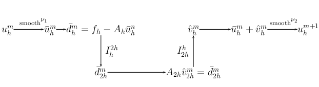
Multigrid techniques provide optimal, or near-optimal, and highly efficient solvers for a broad set of linear and non-linear equations which are usually derived form several classes of partial differential equations. The optimality of the multigrid methodology results from the combination of iterative solvers with grid transformations and is based on two principles: (i) smoothing iterations: short-wavelength error components can be uniformly attenuated with a broad class of iterative procedures, (ii) grid coarsening: a smooth error can be transferred to a coarser grid without significant information loss. Fig. 1 illustrates the basic two-grid iteration which can be applied recursively in a variety of combinations.
Besides adaptivity, generality and high efficiency, another important feature of multigrid for today's computer architectures is the possibility to use algorithms with multiple levels of parallelism, e.g.: the grid over which the solution is sought can be partitioned to MPI tasks which exchange only halos with their topological neighbours, the update operation for smoothing, restriction and prolongation can be parallelised further with OpenMP threads [4].
The main components of DL_MG were selected following the standard
recommendations for the PE and PBE. The grid stencils are derived by
discretisation of the differential operator at each level (geometric
approach) with the finite differences method. In order to generate the
multigrid levels, the global grid must have sizes given by
[q12n1 +1, q22n2 +1, q32n3 + 1] with
q1 ![]() q2
q2 ![]() q3
q3![]() 20 for an efficient solution at the coarsest
level. Coarsening is achieved by doubling the lattice constant in all
dimensions, smoothing uses Gauss-Seidel red-black method, inter-grid
transfers are performed with half-weight restriction and bilinear
interpolation. The non-linear case (PBE) uses the full approximation
scheme (FAS). With the above components one can build a close to
optimal and efficient solver for the PE and PBE, provided that the
models used for the permittivity and charge density are smooth and
without strong anisotropies [4].
20 for an efficient solution at the coarsest
level. Coarsening is achieved by doubling the lattice constant in all
dimensions, smoothing uses Gauss-Seidel red-black method, inter-grid
transfers are performed with half-weight restriction and bilinear
interpolation. The non-linear case (PBE) uses the full approximation
scheme (FAS). With the above components one can build a close to
optimal and efficient solver for the PE and PBE, provided that the
models used for the permittivity and charge density are smooth and
without strong anisotropies [4].
The V-cycle was selected for multigrid iterations as generally recommended for parallel computations [4,5]. MPI parallelism is used for data decomposition; the cuboid global grid is distributed amongst MPI ranks using a 3D topology. As the coarse grids are derived from the fine grids by removing the points with even index coordinates in all directions, no data is exchanged between MPI ranks during inter-grid transfers. The number of MPI ranks can vary across multigrid levels because some ranks could be assigned zero grid points below a certain coarsening level, depending upon the global grid size and MPI topology at the finest level. MPI communication at each level is done in a separate communicator that includes only the active ranks. The solver is provided with the option to ''agglomerate'' the grid domains at a chosen level and thus to use only one MPI task for the levels below. Domain halos are exchanged with non-blocking send-receives, the edge and corner points of the local domains are transfered between ranks by using ordered communication along axes between nearest neighbours [4].
OpenMP parallelism is implemented using one parallel region that covers the V-cycle loop and the subroutine which builds the stencil coefficients. The local domain is decomposed in thread blocks with an algorithm that ensures equal work for all threads even in the case of very thin local domains (situation encountered in ONETEP in certain use cases). Block sizes can be tuned also for better cache utilisation, if necessary. First touch policy is used to ensure optimal memory access on NUMA architectures. MPI communication inside OpenMP regions is handled by the master thread (the so-called funnelled mode), mainly for reasons of portability. Data transfers between MPI buffers and halos are done using one thread per local grid side with the help of "single" directives.
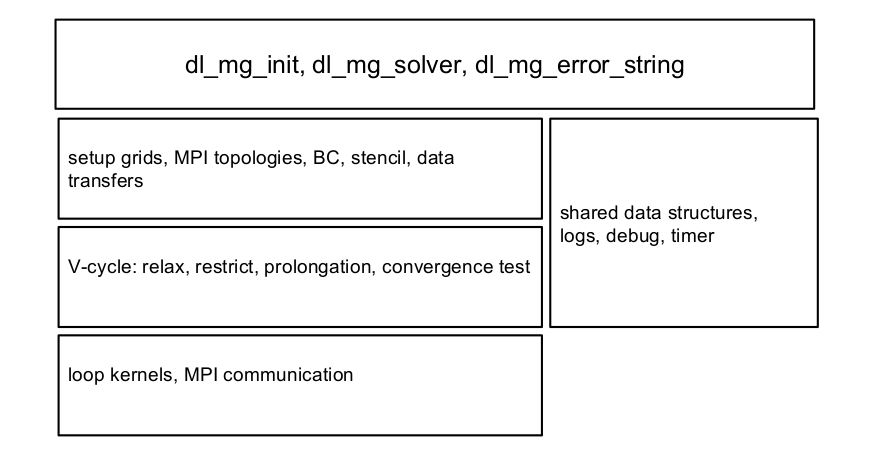
The software package is developed in Fortran 95, uses modules and derived data types for information encapsulation and for maintaining a hierarchal structure of the package. The software stack organisation is sketched in Fig. 2.
Besides the solver subroutines, several auxiliary procedures and programs were developed to ensure solver correctness, to assess its performance and to help its integration with user applications:
 |
 |
DL_MG correctness and performance were thoroughly tested using a three stage procedure.
DL_MG was incorporated in the serial version of CASTEP, the correctness test was passed, the computation efficiency was twice that of the previous multigrid solver. DL_MG non-linear branch for PBE has passed the elementary correctness tests across the various MPI topologies and number of OpenMP threads.
In Sec. A we present more performance data collected on HECToR [16] and IRIDIS4 [17] systems for hybrid parallel mode scaling.
Since August 2013 the DL_MG code (with its updated versions that were developed until the end of this dCSE project) has been included in the ONETEP academic distribution. For the first time this has enabled practical calculations with the solvent model in ONETEP, which is now similar in computational performance to standard "vacuum" calculations, as opposed to being impractically slow before this dCSE project. This has enabled a number of leading research groups in the UK and internationally who use ONETEP to continue their (long overdue) projects which required the solvent model. A selection of these projects is:
Over 15 participants from UK and abroad were trained at the use of the solvent model at the ONETEP Masterclass 2013 which was held in Cambridge between 27-30 August 2013.
In addition to the academic version of ONETEP, the DL_MG code and the solvent model will soon be made available in the commercial version of ONETEP which is marketed by Accelrys and used by researchers in industry.
Overall this project has proved extremely useful for the ONETEP developer and user communities. It is a further demonstration of the success of the HECToR dCSE scheme in enabling the re-engineering of complex algorithms in such a way that they can be run efficiently on supercomputers such as HECToR to benefit their users. While not yet applicable in calculations with CASTEP, this project has made significant progress towards this goal by developing most of the necessary groundwork that will be needed in the future completion of the integration of DL_MG with the solvent model within CASTEP.
The usefulness of this work is not limited to solvation models. An equally useful outcome of the availability of this code within ONETEP and CASTEP is that it also enables their standard (vacuum) calculations to be run under arbitrary (e.g. open) boundary conditions in the form of state-of-the-art real space-based electronic structure theory methods. Up to now the standard implementations of ONETEP and CASTEP relied on Fourier Transforms which necessarily impose periodic boundary conditions. The open boundary conditions make the simulations of molecular and nanoparticle systems more realistic by avoiding the supercell approximation.
Furthermore, beyond the realm of electronic structure theory, the DL_MG library (which will be made freely available via a BSD-type license) will find application in fields such as materials simulations with classical force fields (there are already plans for incorporating it into the DL_POLY package), engineering, fluid mechanics and climate modelling as a few possible examples of its wide applicability.
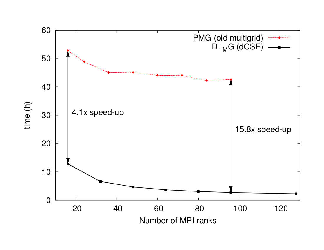
We have delivered a software package thoroughly tested and integrated in the main branch of ONETEP. The performance gain offered by DL_MG with respect to previous solver, a factor of almost 16 at large core counts, allows ONETEP users to explore significantly larger or more complex systems that rely on implicit solvation or open boundary conditions, as detailed in the previous section.
In order help a wider user base, DL_MG is structured as a parallel library package using MPI+OpenMP with a general 3D domain decomposition, hence it can be used easily to solve PE and PBE type of equations in other applications, provided that they have specifications similar to ONETEP or CASTEP.
Nevertheless, more work is needed to complete the unfinished subtasks of this project and to support the computational requirements of future ONETEP and CASTEP projects. Henceforth we plan to continue our work in the following directions in order to enhance DL_MG capabilities and performance:
This project was funded under the HECToR Distributed Computational Science and Engineering (CSE) Service operated by NAG Ltd. HECToR - A Research Councils UK High End Computing Service - is the UK's national supercomputing service, managed by EPSRC on behalf of the participating Research Councils. Its mission is to support capability science and engineering in UK academia. The HECToR supercomputers are managed by UoE HPCx Ltd and the CSE Support Service is provided by NAG Ltd. http://www.hector.ac.uk.
In this section we present more DL_MG performance and scaling data for hybrid parallelism in ONETEP and also for calculations over a grid partitioned in 3D MPI topologies which is representative for CASTEP.
ONETEP uses 1D MPI domain decomposition of its global grid, hence the number of MPI ranks that can be used for parallelism is limited by the number of grid points in the partitioning direction (denoted by z). Furthermore, the thickness of the local domain cannot be reduced to size 1 in the z direction without significant performance loss because of high-order discretisation needed for certain derivatives in the defect-correction procedure (which is a wrapper around DL_MG). In this context, the OpenMP parallelism inside each MPI domain is one of the options that can be used to increase computation parallelism.
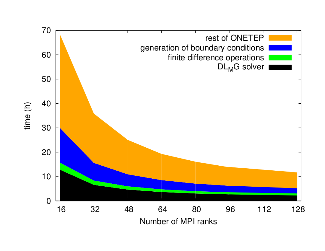
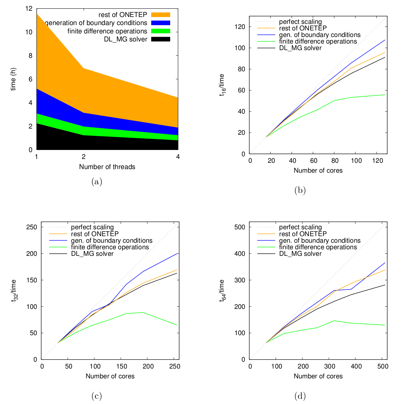
Fig. 5 shows the hybrid scaling performance for ONETEP components used in solvation calculation: DL_MG, boundary condition and defect correction. This set of data was obtained on the IRIDIS4 system [17] using the Intel compiler, with 1, 2 and 4 OpenMP threads, respectively.
For the next benchmark the Poisson problem data were extracted from
the ONETEP lysozyme model and solved separately with DL_MG on HECToR.
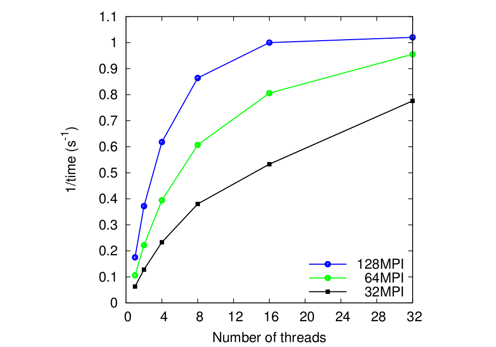
Fig. 6 shows the total solver speed (1/time) for 3
MPI grid partitions to which OpenMP threads are added. The global grid
sizes are:
449 x 545 x 609. The solution was attained in 9
steps for a tolerance of
![]() 10-8, the convergence factor
(the ratio of two consecutive residual norms) was close to 0.125.
Data show that MPI and OpenMP scaling are very good up to 4 threads
for all MPI partitions and acceptable with 8 threads and it stays
positive across the whole NUMA node. DL_MG internal timer was used to
measure the time spent in the multigrid components (smoother,
restriction, prolongation) at each multigrid level for computation and
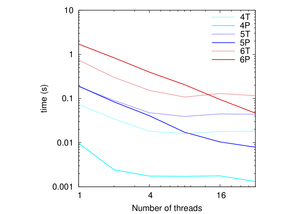
MPI communication sectors. Fig. 7 shows the
scaling of computation and communication for the smoother component,
which takes the largest share of the DL_MG run time (
10-8, the convergence factor
(the ratio of two consecutive residual norms) was close to 0.125.
Data show that MPI and OpenMP scaling are very good up to 4 threads
for all MPI partitions and acceptable with 8 threads and it stays
positive across the whole NUMA node. DL_MG internal timer was used to
measure the time spent in the multigrid components (smoother,
restriction, prolongation) at each multigrid level for computation and
MPI communication sectors. Fig. 7 shows the
scaling of computation and communication for the smoother component,
which takes the largest share of the DL_MG run time (
![]() 70%
amongst multigrid components). Two observations are in order: i) the
communication time decreases with the number of threads inside of a
NUMA node for a 1D grid partition, ii) the degradation of the total
speed scaling in Fig. 6 is correlated with the
loss of scaling for the communication sectors seen in
Fig. 7. This gives us a hint where to focus our
efforts for parallel performance improvements.
70%
amongst multigrid components). Two observations are in order: i) the
communication time decreases with the number of threads inside of a
NUMA node for a 1D grid partition, ii) the degradation of the total
speed scaling in Fig. 6 is correlated with the
loss of scaling for the communication sectors seen in
Fig. 7. This gives us a hint where to focus our
efforts for parallel performance improvements.
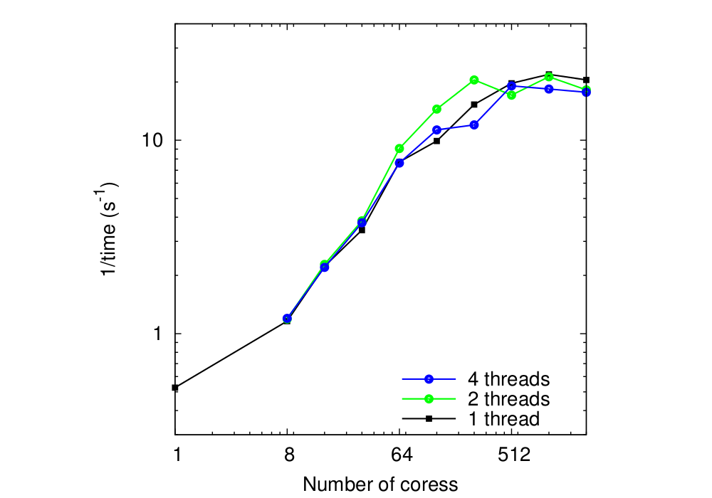
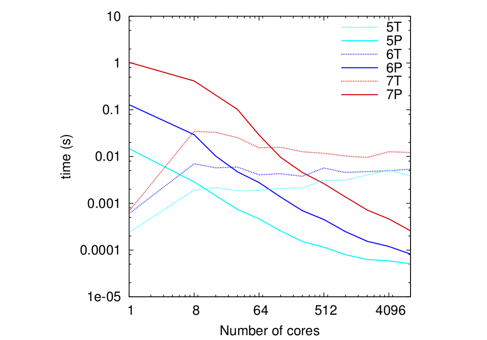
In the last test, done on HECToR as well, 3D MPI topologies were used for global grid sizes 129 x 129 x 129 which is representative for CASTEP calculations. The MPI 3D topologies were build with the following rule
| 2nx x 2ny x 2nz |
 |
 |
 |
 |
 |
This document was generated using the LaTeX2HTML translator Version 2008 (1.71)
Copyright © 1993, 1994, 1995, 1996,
Nikos Drakos,
Computer Based Learning Unit, University of Leeds.
Copyright © 1997, 1998, 1999,
Ross Moore,
Mathematics Department, Macquarie University, Sydney.
The command line arguments were:
latex2html -split 0 -no-navigation -show_section_numbers -html_version 3.2,math -no-math -local_icons -antialias index
The translation was initiated by Lucian Anton on 2013-11-03
