Further Improving NEMO In
Shallow Seas:
Final Report of the dCSE project FINISS
Stephen M. Pickles and Andrew R. Porter, STFC Daresbury Laboratory, January 2014.
Abstract
We describe the motivation, methodology and outcomes of the dCSE project FINISS. Following on from an earlier dCSE project, FINISS aimed to improve the effective load balance of NEMO by eliminating redundant computations on land, using a multi-core aware partitioning method developed for POLCOMS. The approach turns on transforming all 3-dimensional array declarations and references within the code to make the vertical dimension contiguous in memory, and altering loop bounds to avoid traversing the dry points that remain in a sub-domain after partitioning. At the completion of the project, we are able to make an informed estimate of the performance benefits of our methodology extrapolated to full coverage of the NEMO code base, and to comment on the effort required to implement this pervasive set of code changes. We also identify potential improvements that do not depend on these transformations.
Table of Contents
Abstract
1. Introduction
2. Background and motivation
NEMO
Related Work
Decomposition, array index ordering and masks
3. Project structure and timeline
Project plan
Performance targets
Consultation
4. Methodology
5. Results
5.1 Eliminating field values beneath the sea bed from halos
5.2 Reading domain partitioning from File
5.3 Restrict depth loops to the deepest level in each sub-domain
5.4 Loop only over wet levels at each grid point
5.5 Deep ocean benchmark.
6. Conclusions
Discussion
Impact
Recommendations
Acknowledgments
References
Appendix A: stand-alone partitioning tool
1. Introduction
This is the final report of the HECToR dCSE project “Further Improving NEMO In Shallow Seas”.
The goal of the project was to continue to apply a set of modifications to the ocean modelling code NEMO, designed to improve the performance, scalability and usability of the code on modern very large multi-core scalar systems such as HECToR. This work was begun in our first dCSE NEMO project , which is described in full in [9] and summarised here in section 2.
In section 3, we describe the project structure, including sequence of tasks, consultation with stakeholders, and performance targets. Section 4 provides detailed technical information about our methodology, aimed primarily at NEMO developers. Section 5 reports performance results, as achieved by the end of the project. In section 6, we present our main conclusions and recommendations.
2. Background and motivation
NEMO
NEMO (Nucleus for a European Model of the Ocean) [1] is an ocean modelling code of great strategic importance for the UK and European oceanographic communities.
Although NEMO has been used successfully for a number of years in global and ocean basin applications, its use as a shelf-sea model is less well developed. In order to align the shelf-seas modelling work with the open-ocean, to coordinate effort with the Met Office and to address issues of ocean-shelf coupling, the shelf-sea modelling partners of the UK marine research programme (Oceans 2025; see http://www.oceans2025.org) determined to transition from the use of the Proudman Oceanographic Laboratory Coastal Ocean Modelling System (POLCOMS) [2, 3] to the use of NEMO for modelling shelf seas. When making this decision, they recognised that significant work would be required to bring NEMO to bear on Grand Challenge problems in multi-scale oceanography, particularly in the algorithms used for shallow-sea problems and in the performance of the code and its scalability to many thousands of cores on modern architectures.
Related Work
This project builds upon previous work on NEMO and POLCOMS. A dCSE project looked at compiler options, use of netCDF 4.0 compression, and the removal of land-only cells by pre-processing [4, 5]. In the GNEMO project [8] we examined the feasibility of porting NEMO to GPUs.
Hybrid MPI+OpenMP parallelisation strategies (see e.g. [10]) have become increasingly important with the commoditisation of multi-core, shared memory nodes, and early experiments applying this approach to NEMO have been conducted at CMCC [11]. The activity is continued in Work Package 8 of PRACE-2IP, in which alternative approaches to those employed in [11] were investigated.
The issue of I/O performance in NEMO is being addressed by the development of asynchronous, parallel I/O (using XIOS) within the core NEMO programme. This is due to be a part of NEMO version 3.6.
Our own work in the GSUM project [6], and our refinements to the POLCOMS partitioning method [7] in the GCOMS project [3], together established the feasibility of the programme of work started in [9] and continued here.
Decomposition, array index
ordering and masks
Three-dimensional fields in POLCOMS are stored in the z-last ordering, i.e. they are declared as fortran arrays in the style a(z,x,y) with the vertical (z) index varying fastest. POLCOMS deals with the issue of computational load imbalance by decomposing, at run-time, the domain into rectangular sub-domains with approximately equal numbers of wet points, using a recursive k-section partitioning method [2]. Computation on dry points that remain in a sub-domain after partitioning are avoided by explicitly testing whether a point (x,y) is dry. In [7], we extended this method so that a number of alternate partitions are evaluated in parallel, and the best partition (according to a cost-function that takes into account various performance-affecting factors including the placement of MPI tasks on multi-core nodes). We refer to this method as multi-core aware partitioning.
In contrast, 3D fields in NEMO are stored in the z-last ordering, i.e. they are declared as fortran arrays in the style a(x,y,z) with the vertical (z) index varying slowest. NEMO decomposes its domain into equally sized rectangular sub-domains, applies the same computations on both wet and dry points, and masks out the results of the redundant computations on dry points using 3D mask fields, applied multiplicatively. There is much redundancy in this representation, which leads to an effective load imbalance equal to the fraction of dry points in the global domain, but the NEMO approach is certainly well suited to vector architectures.
The dCSE NEMO project [9] aimed to improve the performance and scalability of NEMO, especially for limited area, shallow-sea problems, where the fraction of dry-points in the domain can be as high as 50% or so. It is important to note that it is only practical to avoid computation on dry points in the z-first ordering, where the overhead of testing whether a point (x,y) is on land can be amortised over a whole water column. The steps in this programme of work were:
· Introduce multi-core aware partitioning and halo-exchange optimisations into NEMO;
· Transform all 3D array declarations and references from the z-last ordering to the z-first ordering, using the fortran pre-processor FTRANS [12];
· Manually permute loop nests for better cache reuse in the z-first ordering;
· Further manual transformations to avoid looping over the dry points that remain in a sub-domain after partitioning.
The result of this work was a branch of the NEMO source tree that could be pre-processed either to produce a z-first version or recover the original z-last version. Unfortunately, we had under-estimated the work involved in implementing these pervasive and extensive changes, which touched almost every NEMO source file. Consequently, we did not have enough time left to implement the important step of eliminating the redundant computation on dry points that remain in a sub-domain after partitioning, and the load-balance was limited by the size of the largest sub-domain, instead of the highest number of wet points in any sub-domain.
During the dCSE NEMO project, we realised that NEMO also performs redundant computation and communication on field values located beneath the seabed. This arises because in some of the supported vertical co-ordinate schemes, the number of active levels at each point (x,y) varies across the domain.
3. Project structure and
timeline
Project plan
The principal aim of the follow-up project FINISS was to eliminate the remaining redundant computations on land, sufficient to enable a properly informed estimate of the performance benefits and the effort required to achieve them. Secondary aims were to reduce redundant computation and communication on field values beneath the seabed, and where possible, to do this in both the z-first and z-last orderings.
We were awarded funding for 6 person-months of effort. Due to prolonged staff illness, the project ran for 12 months (instead of the planned 8), completing in December 2013.
Our project plan consisted of four work packages, as
originally stated:
1. Reduce the bandwidth requirements of halo exchanges for 3-dimensional fields by eliminating from halo messages field values beneath the seabed. This will be implemented in both the z-first and z-last orderings.
2.
Add an optional
facility in NEMO to read in the partition information from a file, which would permit the use of off-line
generated "grid-partition" maps. The maps will be human-editable,
enabling the hand-tuning of partitions
for long production runs.
3.
Determine the deepest
level in each processor’s sub-domain, and restrict the outer loops over the vertical dimension so that lower levels (which are beneath the seabed) are not traversed. Although this transformation does not promise
as much as the transformation of task 4 (see below), it
is considerably less invasive and it works in the existing
z-last ordering.
4. Improve load-balancing and cache re-use in key routines using the z-first ordering, by looping only over active levels at each grid-location, eliminating redundant computations on land and beneath the sea bed. The routines will be selected in order of the contribution to NEMO’s profile, as reported by CrayPat on HECToR. We would expect to transform 10-20 routines, accounting for >50% of the run-time, during this work. This should be sufficient to make reliable extrapolations of performance benefits and the effort required to apply similar transformations to the whole of NEMO, thereby enabling an informed recommendation to the NEMO developers. We will use the AMM12 configuration, a limited area model surrounding the British Isles, both for testing and performance measurements.
The order of work packages was devised to minimise risk by tackling more straight-forward tasks first.
Since this work relies upon that completed in our previous dCSE project, we continued to work with the same version of NEMO. This was originally forked from NEMO v.3.3.1 in January 2011 and has its own branch in the NEMO Subversion repository. All of the code developed in this project was committed back into this repository, and is available to the NEMO consortium.
Performance targets
The likely performance benefits of this work were difficult to quantify at the outset. This is because they will vary according to the fraction of dry points in the domain, the bathymetry and the vertical co-ordinate system used, and the efficiency of the load-balancing scheme. For seas surrounding the UK, the maximum gain achievable is determined by the elimination of land points (around 50%) and levels beneath the seabed. Based on experiences with POLCOMS, in the z-first ordering it should be possible to achieve within 5-10% of the maximum possible saving, the short-fall being due to imperfect load balance. It was not possible to quantify this for the z-last ordering until we had some idea of the number of levels beneath the sea bed.
Consultation
We consulted with project partners and external stakeholders. In particular, we:
· made regular visits to the National Oceanography Centre (NOC);
· attended the 2013 meeting of the NEMO Extended Developers Committee;
· liaised with external projects and organisations with an interest in NEMO, including PRACE (1IP and 2IP), EC-EARTH/IS-ENES, CMCC (Lecce) and the NERC Ocean Roadmap Project.
4. Methodology
In order to exclude land points from calculations in NEMO, we have introduced a new array, mbkmax, and used it to store the index of the last level above the ocean floor at each grid point. This array is then used in place of jpk as the upper bound of DO loops over levels. This has the advantage of not introducing any additional conditional statements to those already implicit in the DO loop construct.
We applied this transformation to a total of 25 source files. These source files were selected on the basis of CrayPAT profiles taken on a run on 90 MPI processes; the total time spent in the associated routines accounted for 90% of the time spent in user code (that is, excluding I/O and MPI functions).
Although most of the code changes were straightforward, we did have to take care with the boundary conditions applied at the bottom of a water column in some routines (e.g. tra_zdf_imp which deals with vertical diffusion). These conditions had to be applied at level mbkmax instead of jpk.
A drawback of this approach is the fact that mbkmax(:,:) is never less than one, even over land. (This is necessary because NEMO occasionally uses jpk to index directly into an array, and replacing it with mbkmax would cause out-of-bounds array accesses for those points if mbkmax were set to zero.) Therefore all depth loops will have a trip count of at least one, with the associated penalty of loading from memory any variables used within them.
The alternative approach, of testing a two-dimensional, logical mask for land points before looping over the vertical dimension would avoid this issue, at the price of more intrusive code modifications. This is the approach adopted in POLCOMS.
In order to estimate the overhead of replacing jpk by mbkmax(ji,jj) in loop bounds, we compared the performance of the two methods on a configuration with no land. We did not observe a measurable difference in performance, and we conclude that the overhead is negligible.
5. Results
In the following, we describe the results obtained from each of the four tasks in the project work plan.
5.1 Eliminating field values
beneath the sea bed from halos
Halo exchanges in this (recursive, k-section partitioning) version of NEMO have previously been optimised to reduce the number of dry points being communicated between processes. This is achieved by breaking each halo up into patches of contiguous wet points and communicating only those patches. In this work we extended the description of these patches to include a depth, set to be the maximum depth of any water column in the patch.
Testing this functionality on the AMM12 configuration revealed that the savings achieved were disappointing – typically the reduction in the number of data points to be exchanged between processes was only of the order of one percent. We attribute this to the hybrid z-s coordinate scheme used for the vertical levels in this configuration. This scheme adjusts the vertical resolution of the grid according to the ocean depth, thus minimising the number of vertical levels beneath the ocean floor. Savings are likely to be greater if a less-sophisticated z-coordinate scheme is used.
5.2 Reading domain partitioning
from File
The new functionality is activated by use of a new field, nn_readpart, in the &nammpp section of the namelist file. Setting this to .TRUE. now causes NEMO to read in a partitioning from a file ‘partition.dat’ in the current working directory. The format of this (ASCII) file is described in Appendix A.
A stand-alone tool has been created to produce this partitioning file and is included in the SVN branch containing the modified version of NEMO. More details about this tool are given in Appendix A.
5.3 Restrict depth loops to
the deepest level in each sub-domain
We implemented this functionality by overwriting the variable jpk, which holds the number of vertical model levels. (The original value of jpk is stored in a new variable, jpkorig.) This is done once the domain decomposition is complete and the majority of arrays have been allocated (i.e. after the call to nemo_alloc()). Unfortunately, calling nemo_alloc() does not result in the allocation of all arrays that have an extent determined by jpk. Some debugging was therefore required to find the remaining allocate statements and replace their use of jpk with jpkorig. Care also had to be taken with the routines concerned with I/O as they perform special actions with arrays that have had their indices re-ordered by ftrans (because we preserve the data ordering in the files read/written by NEMO).
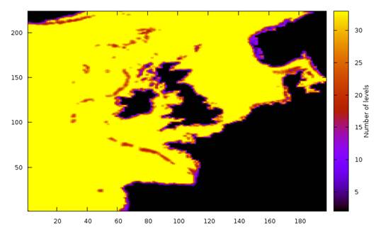
Figure 1: the number of vertical levels above the sea floor at each grid-point in the AMM12 configuration.
Figure 1 shows the number of vertical levels above the sea floor for each point in the AMM12 configuration. As with the halo optimisation, it turns out that using the hybrid z-coordinate scheme causes the majority of grid points to retain the full number of vertical levels (33 in this case) above the sea floor. However, there are areas where the number is reduced, particularly along coastlines and around the edge of the continental shelf.
5.4 Loop only over wet levels
at each grid point
Our recursive k-section partitioning algorithm assumes that dry points do not have any computational cost and therefore counts only wet points. The fact that in our previous dCSE project we were unable to add the ability to exclude residual land points from computational loops meant that load imbalance had become a problem. As an example, the decompositions obtained for the AMM12 domain on 128 processes by the recursive k-section and the default NEMO algorithms are shown in Figure 2.
Trimming off the land-only areas in the decomposition in Figure 2(a) has resulted in sub-domains that are generally smaller than those in the regular example in Figure 2(b). However, there are some sub-domains (such as numbers 57 and 122) that are much larger than the average (e.g. 74) because they contain land.
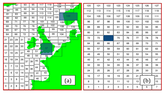
Figure 2. Comparison of the domain decompositions produced by the recursive k-section algorithm (a) and the original NEMO code (b) for 128 processes. Sub-domains highlighted in blue illustrate the load-imbalance problem in (a).
In this work package we have now altered the code to exclude calculations on dry points, as described in the Methodology section.
In Figure 3 we compare the performance of this new, ‘FINISS’ version of NEMO with that of the original for the AMM12 configuration. For reference, we also show the performance of the code as it was at the end of our previous dCSE project. It is clear that the performance of FINISS-NEMO is considerably improved over that of dCSE I, especially on more than 100 PEs. However, it is also clear that these gains have only made the performance of FINISS-NEMO comparable to that of NEMO using a regular domain decomposition and z-last ordering.
We investigated the performance of FINISS-NEMO and original NEMO in some detail on 224 PEs – a PE count on which original NEMO is some 10% faster. Experiments with craypat showed that approximately 40% of the run-time is spent in MPI routines in both cases. It also showed that the key difference between runs with the two binaries was the time spent in the dyn_spg_ts routine. This routine uses a split-stepping method to evolve the free oceanic surface forwards in time. From a computation view point, it has three significant properties:
1. it works only on two-dimensional fields since it deals with the ocean surface;
2. it loops over many (~30 in AMM12) sub-time steps in order to evolve the fields forwards for a single model time step;
3. each iteration of the sub-time step loop involves halo exchanges for five, two-dimensional fields.
As a consequence, the performance of dyn_spg_ts is very dependent upon the performance of halo exchanges for 2D fields. In fact, for an 800-time-step run of the AMM12 configuration, craypat showed that dyn_spg_ts accounted for 95% of the MPI messages originating from 2D halo swaps and 83% of the total MPI message count.
Comparing the two runs, craypat also showed that while the total quantity of data communicated via MPI in the FINISS case was 13% less than with the original version, it also communicated 70% more messages. This increase in messages is an unfortunate consequence of the particular domain decomposition created for this PE count, which results in a need to transmit sub-domain corner points between diagonally-neighbouring sub-domains. The irregular domain decompositions generated using the recursive k-section partitioning can also introduce more of a communications imbalance than can a regular decomposition. In the latter, a processor in the corner of a limited-area configuration may only have to communicate with two neighbours and the maximum number a PE must communicate with is four. In the recursive k-section case on the same configuration, the minimum number remains two but the maximum number is now eight (four sides plus four corners).
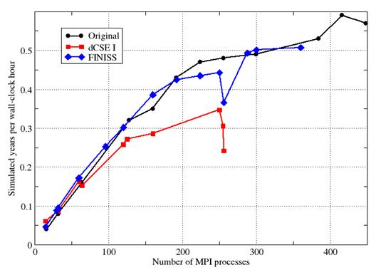
Figure 3. Performance comparison of three versions of NEMO with the AMM12 configuration on Phase III of HECToR. ‘Original’ denotes the FINISS source code built with z-last (normal) index ordering and regular domain decomposition. ‘dCSE I’ denotes the performance obtained at the end of the previous dCSE project while ‘FINISS’ denotes the performance obtained after all of the modifications made in this work.
We note that the original NEMO avoids the need for separate corner-point messages in halo exchanges by requiring that east-west exchanges complete before the north-south exchanges commence. In contrast, FINISS allows east-west and north-south exchanges to proceed concurrently, and must provide for the possibility of separate corner-point messages. In principle, a small tweak to the FINISS partitioning method should reduce significantly the number of separate corner point messages.
While halo exchanges for three-dimensional arrays go significantly faster in the z-first ordering [9], we gain no such performance benefit for two-dimensional arrays and so the large increase in message count associated with them in the FINISS version causes a reduction in overall performance. We know from our previous work in the GSUM project [6] that it is possible to optimise cases where several consecutive halo exchanges take place by packing together the halos for the different fields and exchanging them all at once. In subsequent work [7] we found that packing the halos of 2D fields could result in doubling the effective rate of halo exchange. For halo exchanges on 3D fields, which are limited not by latency but by bandwidth, the situation is less clear; combining 3D halo exchange operations brings little benefit and can actually reduce performance in some cases [7]. Since the five 2D halo exchange calls within the sub-time-stepping loop in dyn_spg_ts are split into two groups; one of three consecutive calls and the other of two consecutive calls, they could effectively be replaced by two, packed halo swaps. This would be a significant optimisation in both the original and FINISS versions of NEMO for any configurations that use the time-splitting approach with a free ocean surface.
5.4.1 Tuning the
Multi-Core Aware Cost Function.
At the heart of the Multi-Core Aware (MCA) domain decomposition is a cost function which is used to score the various decompositions that are possible on a given process count. At the end of our previous dCSE project we had to increase the weight given to the computational cost of land points in a sub-domain, wland, from 0.02 to 0.9. However, now that we are excluding the majority of calculations on land points we are in a position to re-visit this issue.
The scoring function we use is that described in [7], extended to attempt to account for resource contention when communicating off node. (This became an issue when HECToR upgraded to the number of cores on a single node without a proportional improvement to the network interface.) As such it takes the form:
Score = Overall + Node_comms + Total_comms
where:
Overall = MAX over all PEs (PE_overall_score)
PE_overall_score = wwet.Nwet + wdry.Ndry + wpli.pli + wplx.plx + wpci.pci + wpcx.pcx
Total_comms = wtil.tli + wtlx.tlx + wtci.tci + wtcx.tcx
Node_comms = MAX over nodes(Node_comm_score)
Node_comm_score = wnli.nli + wnlx.nlx + wnci.nci + wncx.ncx
tli = SUM over nodes(nli)
tlx= SUM over nodes(nlx)
nli=SUM over PEs in node(pli)
nlx = SUM over PEs in node(plx)
pli = SUM over PE boundary pts(Data points communicated to PE on same node)
pcx=SUM over PE boundary pts(Distinct PEs not on same node to communicate with)
etc.
In these expressions, Nwet is the number of wet points belonging to a PE, Ndry is the corresponding number of dry points and the wxxx are weighting parameters. The values for these weights are listed in Table 1.
|
Weighting parameter |
Value |
|
wwet |
1.0 |
|
wdry |
0.9 |
|
wpli |
0.01 |
|
wplx |
0.2 |
|
wpci |
0.5 |
|
wpcx |
10.0 |
|
wnli |
0.0 |
|
wnlx |
0.2 |
|
wnci |
0.0 |
|
wncx |
10.0 |
|
wtli |
0.0 |
|
wtlx |
0.01 |
|
wtci |
0.0 |
|
wtcx |
0.5 |
Table 1: The values used or the weighting parameters in the MCA scoring function.
Figure 4 shows the performance (both of halo exchanges and of NEMO overall) of the various possible partitions on 192 PEs. The partitions are ordered according to their cost-function score with the highest-scoring partition on the right. The weighting of dry points is kept unchanged from its value in dCSE I, i.e. wdry=0.9.
The upper plot in Figure 4 shows the performance of NEMO at the end of the previous dCSE project (with z-last ordering) and the lower plot shows the current performance of NEMO (‘FINISS-NEMO’) with z-first ordering. It is clear that halo-exchange performance is generally considerably better in the FINISS-NEMO plot, sometimes by as much as 100%. Since we have already established that the trimming of halos to remove points beneath the sea floor has little effect (Section 5.1), this must be due to the change to z-first ordering, which is favourable for halo exchanges of 3D fields because columns are contiguous in memory. NEMO performance as a whole (time-steps per second) has also increased but it has done so in such a way as to reduce the gap between the worst and best performing decompositions. It is also clear that the cost function is less able to predict the relative performance of the decompositions – it correctly identifies the best partition but the second best is down in 9th place.
The obvious next step is to reduce the value of wdry to allow for the fact that we are excluding the majority of calculations over land points. However, we experimented with values of 0.7, 0.5, 0.2 and 0.05 for this parameter and found no improvement in the predictive power of the scoring function. We investigated this further by examining the behaviour of the various components used to construct the scoring function, as shown in Figure 5. The x-axis of the various plots in this figure is the actual rank of the partition, as obtained by performing three runs with NEMO with each partitioning and taking the best measured performance (in terms of time-steps per second rather than just halo exchanges). Therefore, the partitioning with rank 1 performs best and that with rank 12 performs worst. We then plot the values of the different components of the scoring function as evaluated for the given partitioning and look for correlations.
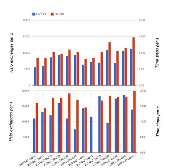
Figure 4. Performance of possible partitions on 192 processes. Top: at end of previous dCSE with z-last ordering. Bottom: current code with z-first ordering. Partitions are ordered according to their MCA cost-function score such that the partition with best predicted performance is on the right and the worst on the left.
The most obvious correlation occurs for the number of dry points contained in a partitioning: in general, the more dry points a partitioning contains, the worse it performs. This is to be expected since we have not tackled land-point elimination for the entire code base and even in the routines where we have, there is still some residual cost associated with land points, as discussed in Section 4. Both of these factors will result in something of a load imbalance that the current MCA cost function does not take into account. Of the other quantities, pli (length/quantity of data communicated by a processor internal to a node) also appears to show some correlation, with those partitions where this quantity is higher performing worse. Surprisingly perhaps, there is no clear correlation between message counts and performance although since pcx (count of messages sent inter-node by a processor) and pci (count of messages sent intra-node by a processor) each only take one of two integer values this is hard to assess. However, the top three best partitionings have pcx=4 and the two worst have pcx=5 which is reassuring given that we expect messages exchanged internally (between PEs on the same node) to be less costly than those exchanged between nodes.
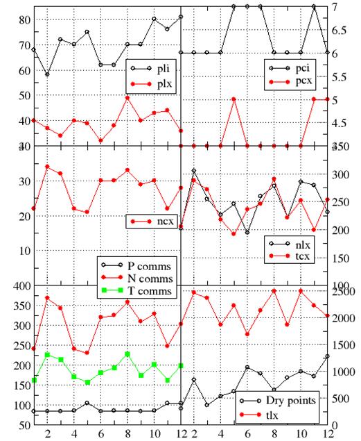
Figure 5. Function constituents against actual rank of associated decomposition for the practical decompositions possible on 192 PEs. Mnemonics: (p)rocessor, (n)ode, (t)otal, (l)ength of data communicated, (c)ount of distinct messages, (i)nternal to node, e(x)ternal to node. Bottom-left plot shows total (P)rocessor comms score, total (N)ode comms score and the (T)otal comms score.
Unfortunately, an in-depth investigation of the MCA scoring function is beyond the scope of this project and will be addressed in future work.
5.5 Deep ocean benchmark.
Finally, we consider the effect of the FINISS modifications on the GYRE test case, which contains no land. In this case, the decomposition selected by FINISS is equivalent to the regular domain decomposition used by the original NEMO, so any differences in performance will be due either to the choice of index ordering or to the different communications mechanisms. Results are shown in Figure 6.
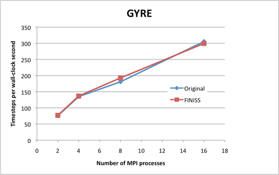
Figure 6. Performance comparison of the original NEMO with FINISS version on the GYRE (deep ocean) test case on a single node of Phase III of HECToR. ‘Original’ denotes the FINISS source code built with z-last (normal) index ordering and regular domain decomposition. ‘FINISS’ . denotes the performance obtained after all of the modifications made in this work. Speeds are quoted in timesteps per second, based on the fastest of three runs for each version.
On two and four MPI processes, FINISS performs 1.5% faster than the original NEMO. On 8 MPI processes, FINISS performs 6.5% faster. On 16 processes, the original NEMO is the faster, by 2%. We explain this in terms of two competing effects. Overall, the z-first ordering used by FINISS tends to result in better cache utilization, and this effect actually increases with the number of MPI processes as competition for memory bandwidth within a multi-core node increases. On the other hand, the maximum number of messages that any process has to send when exchanging haloes behaves worse in the FINISS case, and by 16 processes this effect dominates.
|
Number of MPI Processes |
Maximum number of messages sent by any process |
|
|
NEMO |
FINISS |
|
|
2 |
1 |
1 |
|
4 |
2 |
3 |
|
8 |
3 |
5 |
|
16 |
4 |
8 |
The difference in the two columns is due to corner point messages between diagonally adjacent sub-domains.
The z-first ordering brings a measurable improvement in performance due to better cache utilisation on commodity processors. The effect, albeit minor, is sufficient to outweigh the better vectorisation of tri-diagonal solves in the z-last ordering (at least on HECToR, whose processors have limited instruction level parallelism). The corner point messages could be eliminated, by a small perturbation to the domain decomposition.
6.
Conclusions
Discussion
In principle, full elimination of redundant computation on dry points should bring performance improvements equal to the fraction of dry points in the domain, which varies from about 20% for a global model, up to around 50% for limited area models such as those used operationally by the Met Office and the National Oceanography Centre for the seas surrounding the British Isles. In practice, the performance savings will be somewhat less than this, due to the impossibility of achieving perfect load balance. However, the POLCOMS experience leads us to believe that 90% load balance can readily be achieved, and it would not be unreasonable to hope for 95% given some hand-tuning of the domain decomposition (for example, using the stand-alone partitioning tool) for operationally important configurations. So a reasonable performance target would be a 45% reduction in run-time on configurations such as AMM12 (excluding I/O).
At the end of this work, it is clear that the performance of FINISS-NEMO falls short of this target. We now consider the reasons for this shortfall, and the extent to which it could be alleviated with further work.
One reason is the fact that the loop-level elimination of dry points is not complete. This impacts performance adversely, in several, subtle ways. Most importantly, routines with loop-level dry-point elimination will have different load-balance characteristics than those without. At various synchronisation points such as halo exchanges or global reductions, the accumulated load imbalance from the routines without dry-point elimination will manifest as delays waiting for an MPI operation to complete. This shows up in profiling statistics as an apparent load imbalance in MPI. Having performed this profiling experiment, we estimate the typical overall load balance of FINISS-NEMO as 70%. This is significantly less than the naïve estimate of 81% obtained by multiplying the goal of 90% load-balance by the 90% coverage of dry-point elimination. Nonetheless, extrapolating to 90% load balance at 100% coverage of dry-point elimination still seems reasonable.
We have already mentioned a drawback of our methodology (section 4), which results in at least one trip around every vertical loop, and the wasted cache loads that this entails. This must bring some penalty, which we have neither attempted to quantify nor alleviate. However, the penalty should become proportionally less as the number of levels is increased (the 33 levels used in AMM12 is low, and future operational models are likely to use more than twice this number).
Another factor inhibiting the performance of FINISS-NEMO is the fact that we have not attempted to eliminate the references to masks inside loop bodies. In principle, FINISS-NEMO should not have to multiply by a mask to restore zeroes on dry points. In this work, we chose not to eliminate the mask references because it would have required modifying the bodies of almost every loop, and increased the testing and debugging effort considerably. The consequence is that FINISS-NEMO performs not only redundant multiplications inside every loop body (which should be negligible), but also redundant loads on mask arrays (which will not be negligible, as they increase the pressure on the cache hierarchy).
We were surprised by the number of corner point messages in halo exchanges in FINISS-NEMO on AMM12. These occur when sub-domains are diagonally adjacent, such as sub-domains 0 and 3 in Figure 2 (left). In our earlier experiences with POLCOMS on the High Resolution Continental Shelf (HRCS) configuration [2, 7], such messages were extremely rare, and the MCA cost function calculation could ignore them when counting messages. On AMM12, which extends further to the south and west than HRCS, they occur more often in candidate partitions, and the MCA cost function, being unaware of them, underestimates the communication costs of some partitions. So there is scope for improving our Multi-Core Aware partitioning algorithm in this respect. Even in domains with no land at all, it should be possible to find partitions without corner point messages in most cases.
As reported in [9], the transformation to the z-first ordering affects the performance of various NEMO routines in different ways. On HECToR, most operations perform equally well in either ordering. A few strongly favour the z-first ordering, the archetypical example being halo exchanges on 3D fields. Similarly, there is one important class of operation that favours the z-last ordering, that is, a tri-diagonal solve in the vertical dimension.
Tri-diagonal solves deserve a brief discussion here, but a full treatment is out of scope. They occur in several NEMO routines, such as tracer advection. There is a different tridiagonal system to solve on each water column. The problem is the dependencies between iterations in the forward and backward passes of Thomas’ algorithm, which inhibits vectorisation in the vertical dimension. In the z-last ordering, it is possible to vectorise over the horizontal dimensions, with the loop over vertical levels outermost, and NEMO is written to take full advantage of this. In the z-last ordering, this approach is extremely cache-unfriendly. In the z-first ordering, these routines can be re-written to have the vertical loop innermost. This simplifies the code, eliminates vector temporaries, improves cache re-use, but still performs poorly, due to pipeline stalls. In other on-going work [13], we have examined several methods aimed to improve utilisation of the processor’s pipeline and/or SIMD execution units, including methods designed to trade-off increased floating-point operations account for better opportunities to exploit instruction level parallelism in the processor. Some of these methods show promise. “Ends-towards-centre” (sometimes called “Burning At Both Ends”) schemes improve pipeline utilisation, but as there are only two “ends”, they cannot fully occupy SIMD execution units with 4- or 8-way parallelism; furthermore, the benefits diminish as the number of levels increase, as the two ends become further apart in memory. Strip-mining the horizontal dimension in blocks of 4 brings an improvement on some compiler/platform combinations (including HECToR), but not all. We have tried sub-structuring methods, trading increased floating-point operations for increased (instruction-level) parallelism, but it in practice it is difficult to cajole compilers into emitting SIMD instructions, and the additional flops are not free. So while there is definitely scope to improve the performance of tri-diagonal solves in the z-first ordering, we have not found a method that reliably does so on all problem sizes, compilers and platforms.
It is tempting to speculate about how architectural trends might change this picture. If increasing core counts make the case for MPI+OpenMP hybridisation compelling, then the z-first ordering has advantages in the strong scaling limit [8]. On the other hand, any increase in instruction level parallelism within commodity processor architectures would tend to favour the original NEMO, because tridiagonal solves vectorise better in the z-last ordering.
We should remark here that the slow increase in Instruction Level Parallelism in commodity processors since the 1990s appears to have vindicated NEMO’s perseverance with a coding style that favours vector architectures. We suspect that much of the “traditional wisdom” linking the z-first ordering to better performance on scalar processors dates back to the 1990s, when the instruction level parallelism in commodity processors was limited to fused multiply-add instructions.
In summary, we think that our original performance target of a 40% reduction in run-time on a shallow sea test case (50% land) can be achieved, by completing the implementation of loop-level avoidance of dry points, and making minor improvements to FINISS’s partitioning algorithm. To do better than this, it would be necessary either to find an effective recipe for the tri-diagonal solves, and/or to find other opportunities for optimisation in the z-first ordering (this is not unreasonable, given that NEMO’s idiom is so well adapted to the z-last ordering).
However, to claim a 40% reduction in run-time on shallow sea configurations would not be a fair comparison with the original NEMO. This is because NEMO has a facility to identify sub-domains that only contain land points, allowing a subsequent run to proceed on a smaller number of MPI processes. If the facility removes say 20-25% of sub-domains from AMM12, then we should be comparing 90% load balance for FINISS-NEMO (extrapolated to 100% coverage of dry-point elimination) with 75-80% effective load balance for the original NEMO. Furthermore, the gap will tend to close as the number of sub-domains increases. Likewise, the gap will be less on configurations that contain a smaller fraction of land in the domain.
So the case for applying the FINISS methodology to the NEMO trunk turns on whether the projected benefits outweigh the effort of the pervasive and intrusive code transformations required. An optimistic estimate of the benefits would be say 15-25% efficiency improvement on shallow sea (based on a 10-15% improvement in effective load balance, and a 5-10% improvement from better cache utilisation and further optimisations in the z-first ordering that are yet to be discovered). A more conservative estimate might be a 10% efficiency improvement, based on effective load balance alone.
The FINISS experience tells us that the effort required to fully implement these code transformations amounts to a science-neutral rewrite. Using tools such as FTRANS can help along the way, but it is not sustainable in the long-term to maintain a code base that supports both the z-first and z-last orderings, because the optimal form of almost every loop’s control structures and body is different in the two orderings. The volatility of the NEMO source tree during the dCSE NEMO and FINISS projects has caused considerable drift between our starting point and the NEMO trunk, making it preferable to start again from the NEMO trunk than to attempt to resolve conflicts in almost every source file. The total effort required is likely to be more than expended in dCSE NEMO and FINISS (which did not cover the entire NEMO code base); the approaches developed in FINISS would help, but there would be a need for considerably more testing than we were able to undertake. Simplifying the code base to remove deprecated options would help somewhat. We estimate that at least 2-3 person-years would be required to make the transition, and think it unlikely that this could be achieved in much less than 12 months elapsed.
Impact
The most immediate impact of this work will be seen in:
1. Identification of the performance bottleneck associated with the great number of halo swaps in the code used to evolve the free ocean surface with the time-split method. We recommend the packing of these halos to significantly reduce MPI message traffic.
2. Further recommendations for future NEMO developments, as detailed below.
3. Feedback into future ocean-model development through the recently-funded NERC project “G-Ocean:2D”, which aims to develop a prototype ocean model based on the technology developed within the Gung Ho project [13].
Recommendations
As discussed in section 5.4, the five 2D halo exchange operations within the sub-time-stepping loop in dyn_spg_ts can be replaced by two combined halo exchange operations, reducing the number of messages. This would be a significant optimisation in both the original and FINISS versions of NEMO for any configurations that use the time-splitting approach with a free ocean surface.
We endorse the proposal [14] to simplify the NEMO source. Over a period of several years, NEMO has steadily taken on an increasing number of alternative methods, some switchable at build time and others at compile time, to a point at which the burden of maintaining and testing an unwieldy set of supported options is preventing strategic development work. During our own experiences in this and our previous dCSE project, we felt that the complexity of NEMO’s supported options and the interactions between them seriously impeded our ability to implement and debug the pervasive code changes required by our programme of work. We therefore welcome the proposal to retire some of NEMO’s supported options.
At the conclusion of this work, we are forced to admit that the case for transforming the NEMO trunk to the z-first ordering is not a compelling one. The effort required (2-3 person years) and a likely 12-month hiatus in the release cycle is a high price to pay for a modest improvement in effective load balance on shallow sea configurations, and a marginal improvement on global configurations.
If the NEMO committee decides that the benefits do not outweigh the effort required and that the limited resources in the NEMO core development team are better deployed on other strategic work, then we have one further recommendation to make. This concerns the existing facility for removing all-land sub-domains, which does not appear to be widely used. We have been given to understand that it is not used operationally by the Met Office. We recommend that the reasons for this are investigated, and if necessary, effort is expended in improving the usability of this facility and addressing any concerns about its correctness. The stand-alone partitioning tool developed in FINISS may be of use here.
Acknowledgments
This
project was funded under the HECToR Distributed Computational Science and
Engineering (CSE) Service operated by NAG Ltd. HECToR – A Research Councils UK
High End Computing Service – is the UK's national supercomputing service,
managed by EPSRC on behalf of the participating Research Councils. Its mission
is to support capability science and engineering in UK academia. The HECToR
supercomputers are managed by UoE HPCx Ltd and the CSE Support Service is provided
by NAG Ltd.
We are
grateful to numerous people for assistance, advice, encouragement and
stimulating discussions. We thank in particular Rachid Benshila, Sebastien
Masson, Claire Levy, and Gurvan Madec of the NEMO team; John Siddorn, Dave Storkey,
and Enda O’Dea of the Met Office; Jason Holt, Andew Coward and Hedong Liu of
the National Oceanography Centre; Italo Epicoco, Sylvia Mocavero and Giovanni
Aloisio of CMCC; Mike Ashworth of STFC; and Stephen Booth of EPCC.
References
[1] G. Madec, “NEMO ocean engine”, 2008, Note du Pole de modélisation, Institut Pierre-Simon Laplace (IPSL), France, No 27 ISSN No 1288-1619.
[2] M. Ashworth, J.T. Holt and R. Proctor, “Optimization of the POLCOMS hydrodynamic code for terascale high-performance computers”, Proceedings of the 18th International Parallel & Distributed Processing Symposium, Sante Fe, New Mexico, 26-30 Apr 2004.
[3] Jason Holt, James Harle, Roger Proctor, Sylvain Michel, Mike Ashworth, Crispian Batstone, Icarus Allen, Robert Holmes, Tim Smyth, Keith Haines, Dan Bretherton, Gregory Smith, “Modelling the Global Coastal-Ocean”, Phil. Trans. R. Soc. A, March 13, 2009 367:939-951; doi:10.1098/rsta.2008.0210
[4] Fiona Reid, NEMO on HECToR - A dCSE Project, 4th May 2009, HECToR web site, http://www.hector.ac.uk/cse/distributedcse/reports/nemo/nemo_final_report.pdf.
[5] Fiona J. L. Reid, “The NEMO Ocean Modelling Code: A Case Study”, Proceedings of the Cray User Group, Edinburgh, 2010.
[6] M. Ashworth and A. Porter, “Towards Generic Scaling of NEMO, the oceanographic component of the Unified Model”, Final Report for the GSUM project, 2009.
[7] Stephen Pickles, “Multi-Core Aware Performance Optimization of Halo Exchanges in Ocean Simulations”, Proceedings of the Cray User Group, Edinburgh, 2010.
[8] A. R. Porter, S. M. Pickles, M. Ashworth, “Final report for the gNEMO project: porting the oceanographic model NEMO to run on many-core devices”, Daresbury Laboratory Technical Reports, DL-TR-2012-001 (2012).
[9] Stephen M. Pickles and Andrew R. Porter, “Developing NEMO for Large Multi-Core Scalar Systems: Final Report of the dCSE NEMO Project,” Daresbury Laboratory Technical Reports, DL-TR-2012-002 (2012).
[10] L. Smith and M. Bull, “Development of mixed mode MPI / OpenMP applications”, Scientific Programming, Vol. 9, No 2-3, 2001, 83-98.
[11] Italo Epicoco, Silvia Mocavero, and Giovanni Aloisio, “NEMO-Med: Optimization and Improvement of Scalability”, CMCC Research Paper No. 96, 2011.
[12] Stephen Booth, “FTRANS User Guide”, 1996.
[13] R. Ford, M.J. Glover, D.A. Ham, C.M. Maynard, S.M. Pickles, G. Riley, N. Wood, “Gung Ho: A code design for weather and climate prediction on exascale machines”, Proceedings of the Exascale Applications and Software Conference, 2013, in press.
[14] “Note on possible system simplification”, NEMO consortium internal memo, 2013.
Appendix A: stand-alone
partitioning tool
The domain decomposition created whenever NEMO is run with recursive, k-section partitioning active is written to a file named partition.dat.new. Such a file can also be generated by using the newly-created, stand-alone tool which we have called make_partition.exe. The source code for this has been put in NEMOGCM/TOOLS/RK_PARTITION. This directory also contains a README file which details how to use the tool.
The stand-alone partitioner requires the user to supply the
bathymetry of the model domain in file bathy_levels.nc
and a NEMO namelist file describing
the job that is to be run with the partition (this is primarily used to get the
z-coordinate options). Running the tool with the ‘-h’ flag gives information on
the flags that the tool supports:![Text Box: HECToR $ ../TOOLS/RK_PARTITION/make_partition.exe -h
Usage: make_partition.exe -d <jpiglo>x<jpjglo> -np <nproc> -c <cores_per_node> [-r] [-cyclic] [-h]
Where: domain is jpiglo x jpjglo in extent
nproc is no. of sub-domains/MPI procs required
cores_per_node is no. of cores per compute node on
machine on which NEMO is to be executed
-r : generate regular (old style) partition
-cyclic : enable cyclic E/W boundary conditions
-h : print this message](index_files/image015.png)
Running the tool generates a domain decomposition that is stored in the file partition.dat.new. This may then be used in subsequent NEMO runs by moving it to the working directory, renaming it to partition.dat and setting nn_readpart = .TRUE. in the &nammpp section of the namelist file. The tool also writes the domain decomposition as a postscript file, domain_decomp.ps, which may be viewed with any postscript viewer e.g. gsview.
The file partition.dat is ASCII and intended to be human-readable/editable so that a domain decomposition may be hand-tuned if desired. The contents of partition.dat are written using the following code:
WRITE(UNIT=it,FMT="(I5,1x,I5)")
jpni, jpnj
DO idom = 1,nprocp, 1
WRITE(UNIT=it,FMT="('Domain: ',I5)") idom
WRITE(UNIT=it,FMT="(I5,1x,I5)") pielb(idom), pjelb(idom)
WRITE(UNIT=it,FMT="(I5,1x,I5)") pieub(idom), pjeub(idom)
WRITE(UNIT=it,FMT="(L5,1x,L5)") pilbext(idom),
trimmed(widx,idom)
WRITE(UNIT=it,FMT="(L5,1x,L5)") piubext(idom),
trimmed(eidx,idom)
WRITE(UNIT=it,FMT="(L5,1x,L5)") pjlbext(idom), trimmed(sidx,idom)
WRITE(UNIT=it,FMT="(L5,1x,L5)") pjubext(idom),
trimmed(nidx,idom)
END DO
An example of the first few entries in the file is shown below:
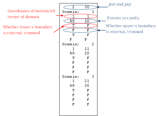
A boundary is described as ‘trimmed’ if it has land-only columns or rows removed so that it no longer lies on a boundary of the global domain (an ‘external’ boundary).