MicroMagnetic modelling of naturally occurring magnetic mineral systems: II
Abstract
This report presents the results of the second HECToR dSCE project to port and parallelise a code (microMag) which models the magnetic properties of mineral systems on to HECToR. This code represents the magnetisation within a structure using vectors located at the vertices of a finite element mesh in order to generate a high-fidelity 3D micro-magnetic model.
The scientific goal of this project is to enable the investigation of large-scale simulations with increased system-size and precision which are currently not possible. These simulations will be of benefit to research into mineral- and palaeo-magnetism.
The key aims of this project are: to complete the parallelisation of the code started in the original project, with particular focus on the generation of the stiffness matrices; and to incorporate a mesh repartitioning algorithm into the code in order to enhance performance.
The PETSc library has been used to provide almost all the required parallel and numerical functionality. Critically, the interfaces it provides to third party libraries such as the adaptive timestep ordinary differential equation solver CVODE and the mesh partitioning library ParMETIS have been utilised.
The outcome of this project is a working, parallelised microMag code on HECToR. A benchmark on a model containing more than 100,000 elements showed speedups of over four times faster on 16 cores.Thus the project has enabled the investigation of large-scale simulations with increased system-size and precision which were previously not possible.
Table of Contents
4.1 Verification and Profiling
4.2 ParMETIS, PETSc and
Partitioning
4.3 Data Conversion Optimisation
1 Introduction
There are many problems in the geosciences that rely on the ability to accurately determine the magnetic properties of minerals and the stability of the palaeomagnetic recordings that they contain. For example, the investigation of the behaviour of the geomagnetic field depends largely on the observed field variations on or above the Earths surface. Temporal records of direct observations stretch back less than two hundred years, and so a more detailed analysis is dependent of ancient recordings made in rocks as they are formed. Geological interpretation of the directional recordings of the ancient field led to the discovery, over 50 years ago, that the Earths oceanic and continental plates are continuously moving. Today, a more thorough understanding of magnetic mineralogy enables a detailed analysis of not only of fine scale continental block motions and rotations, but also emplacement temperatures and thermo-temporal history of the rocks to be determined. In addition, magnetic mineralogy is frequently used as a proxy for determining palaeoclimate variations.
All these applications depend on an understanding of how the magnetic properties of minerals change with the mineral microstructure, chemistry, grain geometry and inter-grain magnetic interactions. The complexity and diversity of naturally occurring magnetic minerals makes the numerical micromagnetic problem a much more difficult task than that applied to the generally more ideal man-made recording media. The increasing sophistication of environmental-magnetic investigations relies on a high-fidelity magnetic re-coding processes occurring in natural magnetic mineral systems. Yet our understanding of the fundamental processes that enable common magnetic minerals to record the local geomagnetic field’s direction and intensity and to retain this information over geological time scales is far from complete. A much better understanding of the recording process in natural materials is required in order to assess the reliability of rock-magnetic recordings.
Equilibrium magnetic domain structures are determined by integration of the Landau-Lifshitz-Gilbert equation of motion. Finite element methods are the preferred technique when dealing with irregular geometries since magnetic domain structures are sensitive to the accuracy with which grain geometries can be modelled. Before the dCSE project the code, microMag, existed as a serial code written in Fortran90. Some initial work had been undertaken in investigating methods of parallelisation. This was the basis for the work-plan submitted as part of the dCSE proposal.
2 Algorithmic details
The numerical micromagnetic model represents the magnetisation within a structure using 3D Cartesian vectors (each of unit length) placed at the N vertices of a finite element (FE) mesh. Tetrahedral elements are employed to reduce the discretisation error. The size of the computational cell is governed by the micromagnetic quantity, termed the exchange length, which restricts the maximum cell size.
Equilibrium magnetic domain structures are determined by a minimisation of the total free magnetic energy of the system, which is achieved by integration of the Landau-Lifshitz-Gilbert (LLG) equation of motion. Dynamical solutions require the LLG equation of motion to be solved for every time step. The total effective field contributions include a computationally intensive non-local (magnetostatic) field calculation, and also the local exchange, anisotropy and externally applied field calculations. Of the previous four component fields only the magnetostatic field is non-trivial. It is also the most computationally intensive part in the determination of the total effective field. A finite volume approach is employed to calculate the exchange and anisotropy fields and is essentially determined by multiplication of the stiffness matrix by the global magnetisation vector.
The magnetostatic field is solved via a scalar potential approach. This requires the solution of the Poisson equation for the divergence of the magnetisation and solution of the Laplace equation for the boundary vertices. An efficient boundary element method is employed to approximate the long-range interaction. Both equations are discretised using a Galerkin scheme for a linear finite element solution of the equations. The solution is obtained via a standard conjugate gradient (BG) solver. The storage required in the solution of the Poisson equation is extremely sparse hence efficient sparse matrix methods are essential. Also, the tetrahedral finite element basis functions provide an efficient way of calculating the remaining three component fields by simple sparse matrix-vector multiplication. Bespoke sparse matrix management is required due to the data layout which arises from the efficient construction of the initial finite element basis functions.
The matrix arising from the boundary element approximation to the long-range interaction is of size , where N is the number of vertices on the material boundary. In a parallel code this dense matrix can be distributed efficiently amongst each individual processing unit. Integration of the stiff system of ordinary differential equations (ODEs) arising from the LLG equation of motion requires an implicit solver and thus requires the approximate inverse to a sparse 3N system of linear equations. The use of explicit methods would be ineffective due the restrictive size of the time-step controlled by the stiffness of the system. The implicit method is a variable order solver which is based on a multi-step backward Euler method with variable coefficients.
3 Work plan
The original work plan for the 6 month project is split into three sections or work packages (WP), and is shown below
WP1 Efficient and accurate construction of the stiffness
matrix code [1 month]
WP2 Parallel matrix generation implementation [2 months]
Task
2a Determine sparseness structure of
each stiffness matrix
Task
2b Create PETSc matrix data objects
with relevant structure
Task
2c Determine matrix values and
populate PETSc matrix objects
WP3 Implement call to ParMETIS for mesh generation [2.5
months]
Task
3a Implement calls to ParMETIS
Task
3b Implement support for alternative
mesh partitions and data decomposition
Task
3c Benchmark the performance of the
code for a large system and write a report
WP4 Final report in html and pdf format [0.5 months]
3.1 Variations from workplan
Chris Maynard was the original member of staff working on this project, but due to a new job left EPCC a few months into the project. Once it was apparent that Chris was leaving Paul Graham was assigned to the project so there was an opportunity to perform a handover, but obviously this had some impact on the technical work as the new staff member needed to get up to speed on the work. The main outcome of this was that the project end date was pushed back and the parallelisation of the matrix generation implementation (WP2) was curtailed.
The impact for not achieving WP2 on the overall success of the project was relatively small, as typically the time spent in initialising the matrix objects is much smaller than the time spent actually performing the calculations. That is not to say that it is not worthwhile doing, but performance optimisation of the calculation phase would clearly reap larger benefits. To this end the WP3 work which could directly affect this was brought forward.
During the project some more detailed profiling of the code was performed, and it was found that one of the performance bottlenecks in the code was a data conversion routine introduced in the previous project. This routine was necessary to convert data to that required by CVODE, but it was inefficient, and thus it was decided that it would be time well spent in optimising this portion of the code.
4 Implementation
Coming into this project, the code was parallelised using MPI, but the initialisation phase is effectively serial. However, even taking this into consideration, the efficiency of the parallel section was very poor and there was still some issues with correctness of results.
4.1 Verification and Profiling
The first part of Work package 1 was to verify that code was producing the correct answer. The results of the serial and parallel code were compared on a benchmark mesh input file. Whilst similar, these outputs were not sufficiently close. However, the serial version of the code uses a preconditioner for the CG solver (which only works in serial), namely an Incomplete Cholesky decomposition. Switching off the preconditioner in the serial code reduced the difference between the outputs. In particular, the resultant vector of the CG solve with preconditioner differed by 3 significant figures, or 1% relative difference to the parallel version: switching off the preconditioner reduced the discrepancy to 12 significant figures. Preconditioning should not change the answer, only how it is computed. However, in such a numerical system, rounding errors can be significant. This effect can possibly be seen for a linear system with a large condition number, or if the rounding errors become significant when computing the preconditioner itself, rather than the CG solve. By systematically replacing the matrices and vectors with the identity or zero, the difference of the serial and parallel code was tracked though the code, and any remaining difference in the original code verified to be numerical rounding error.
Using PETSc self instrumentation features to profile the code revealed it spent large amounts of time in Matrix-Vector operations. Further profiling with the CRAY-PAT tool was performed. It reported large amounts of time were spent in MPI communication routines. This confirmed that the stiffness matrices were responsible for the large amounts of communication and hence slow performance.
The default PETSc data distribution for matrices is by row across the processor ranks. For a sparse matrix, there is a special data structure with a distinction between matrix elements which are in the diagonal block the set of rows which belong to the processor, and those which are off-diagonal. Matrix-Vector operations on the diagonal block are completely local. The off-diagonal pieces require communication. The code was constructing the stiffness matrices, in serial, as FORTRAN arrays, before constructing PETSc distributed data objects and populating them with the values in the FORTRAN arrays. Whilst this is ultimatley a rather inefficient process, it is not the cause per sé of the poor performance when operating with those matrices. They are constructed correctly with the right values.
It was believed that the cause of the poor performance came from the partioning of the mesh, or rather the lack of any formal partitioning. The mesh for any particular geometry is generated by a third party library called Cubit. This is an entirely serial code. Its output is a text file which has the co-ordinates of the vertices, the tetrahedra connectivity list, i.e. what is the vertex number of each vertex of the tetrahedra, and a list of the elements which are on the boundary with how many faces they are connected to. The microMag code knows nothing about partitioning this mesh in parallel. It simply reads in the file, creates the stiffness matrices with the rows and columns based on the values from the mesh file. PETSc then chops these matrices up by row resulting in effectively an arbitrary partition of the mesh. This means that tetrahedra which are connected to each other are distributed across processors. This results in more block off-diagonal than diagonal elements in the matrix and thus potentially a very high communication overhead. Creating a much more efficient partition should help minimise the communication overheads.
This requirement is essentially work package three. In consultation with the code owner it was decided, that as the partitioning is critical to the performance of the code, to bring forward work package 3 and implement the partitioning with ParMETIS before completing work package two. The process employed for this was to first implement a new program to partition the mesh independently. Then the existing microMag code could read the reordered mesh file without further modification, thus allowing for quicker development and testing of the reordering aspect.. Once this was working the partitioning code would then be incorporated into the microMag code so it can be used as a single stage operation.
4.2 ParMETIS, PETSc and Partitioning
PETSc has rather useful feature in that it provides interfaces to several third-party partitioning libraries. ParMETIS is the default partitioning library, and rather than call the native interface to ParMETIS, using the PETSc interface reduces the amount of code integration required at a later stage. The partitioning is done by vertex rather than element.
The methodology for partitioning is:
- Read in mesh data from the PATRAN file
- Convert to a format recognised by ParMETIS
- Generate the new partition using ParMETIS
- Apply the new ordering to the mesh data
- Create the PETSc matrices from the repartitioned mesh
The idea is that the mesh has been well ordered by the repartitioning, so the matrices will also be well ordered, and thus communication will be minimised. There are two new subroutines:
repartVert - this is actually a program used during development which invokes the repartitioning independently of the MicroMag code. It reads in the test model data, and then calls the subroutine reorder, then writes out the newly repartitioned data.
reorder – in this routine, firstly the connectivity data for the vertices is generated, and then used to create the adjacency lists required by PETSc/ParMETIS. The PETSc data structures are then created and the partitioning invoked. The new partition data (which is a list of vertixes with a map of where their new position on the processors is), is then gathered to the rank 0 process, and the partitioning applied, which is effectively a reordering of the vertices and the tetrahedral elements. Finally the vertex and tetrahedra data is broadcast back to the appropriae process elements.
In the main microMag code now has the option of using the partitioning (currently set by a logical variable called usingreordered, it is suggested that a runtime variable may be more useful in the future). If this is set to true, then the reorder subroutine is invoked, and a further step is performed to redetermine the boundary nodes based on the new repartitioning.
4.3 Data Conversion Optimisation
Initial results of the parallel code for both the standard and repartitioned version of microMag were very disappointing, showing no speedup at all as core counts increased, and in some cases going even slower. Closer inspection revealed that one of the causes of this was in two data conversion routines introduced in the previous dCSE project. The microMag code holds the magnetic field in two dif-
ferent data structures. The first is a two-dimensional array of size (NMAX, 3) where NMAX is the number of finite element vertices, and 3 represents the three physical dimensions in Cartesian space. The second data structure is a linearised one dimensional array, (3*NMAX). The code switches between these two data structures several times as the Sundials solver expects a one dimensional array. Looking at detailed timings for the code, this conversion was quite time consuming as in its original form it required several PETSc VecScatter calls, which can carry a significant communication overhead, especially given the frequency with which they were being used. Also, this overhead increases as the core count increases, so any gains in speed seen in the other parts of the code were being countered by the increase in execution time from the conversion routines.
It was considered converting the code in order to maintain the one-dimensional representation throughout, but this would require a fundamental rewrite, so an alternative strategy was employed. Investigation revealed that the conversion between the two representation could be performed entirely locally to each processor – there should be no requirement to send data between cores. Thus two new conversion routines were written so as not to use any communications. Table 1 below shows pseudocode for the old and new conversion routines
Table 1:
comparison of conversion routines
|
Old conversion ! Set up indices ISCreateStride(...)
! 1D stride ISCreateStride(...)
! 3D stride ! Move data
between vectors VecScatterCreate(
... ) VecScatterBegin(
... ) VecScatterEnd( ...
) ! Tidy VecScatterDestroy(...) ISDestroy(...) !Repeat for y and
z ... ! Done |
New conversion ! get local array
values VecGetArrayF90(1dVec,
xyz ...) VecGetArrayF90(xVec,
x ...) VecGetArrayF90(yVec,
y...) VecGetArrayF90(zVec,
z ...) ! move data do i=1, n3d x(i) = xyz(3*i-2) y(i) = xyz(3*i-2) z(i) = xyz(3*i) end do ! Put back in
vectors VecRestoreArrayF90(
...) .... ! Done |
These new conversion routines now of the O(10) times faster than the original routines, and also scaled well with core count. Once this change had been applied parallel speedup was seen in the overall code for the first time.
5 Results
During development three relatively small test cases were used, and one large test case was used for final performance timings:
- brick0_300 – a “brick” shape representing a 300nm size particle, 1826 nodes (8751 elements)
- cube_20nm – a simple cube, 20nm long, 31 nodes, 72 elements
- cube_100nm – a simple cube, 100nm long, 2270 nodes, 10955 elements
- sphere – a sphere , approx 136nm radius, 18838 nodes, 100245 elements
Additionally, the code could be adjusted to run for either a set number of timesteps for each test case, or until the model had converged. Any speedup results reported below are measured against the time taken for the parallel code to run on one core.
As noted earlier initial results for the parallel performance were very poor until the new data conversion routines were introduced. Following the introduction of these, some speedup was seen as discussed below.
Speedup for the smallest test case (cube_20nm) was non-existent, in fact it slowed down on more than one core. This is entirely due to the size of the model, at only 31 nodes there is not enough work to justify the overheads of distributing the data and communications. This test case was primarily used to check for correctness during development as it would take under a minute to run to conclusion.
Figure 1 shows the speedup for two slightly larger test cases, brick0_300 and cube_100nm.
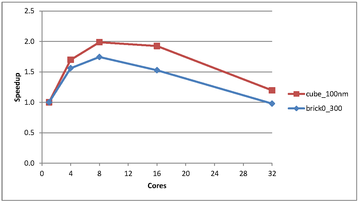
Figure 1: Speedup for the cube_100 and brick_300 test cases
As one can see the speedup is not great, peaking at about 1.7 times faster and 2.0 times faster on 8 cores for the brick and the cube test cases respectively, and then tailing off. For both these cases the time taken for the largely sequential problem initialisation steps were much less than the total execution time (in the order of 0.5% of total execution time) so this was not a contributory factor.
Figure 2 shows a plot of the speedup vs the number of vertices per core after the data has been distributed: this gives an idea of the amount of work each core has to do for these two test cases
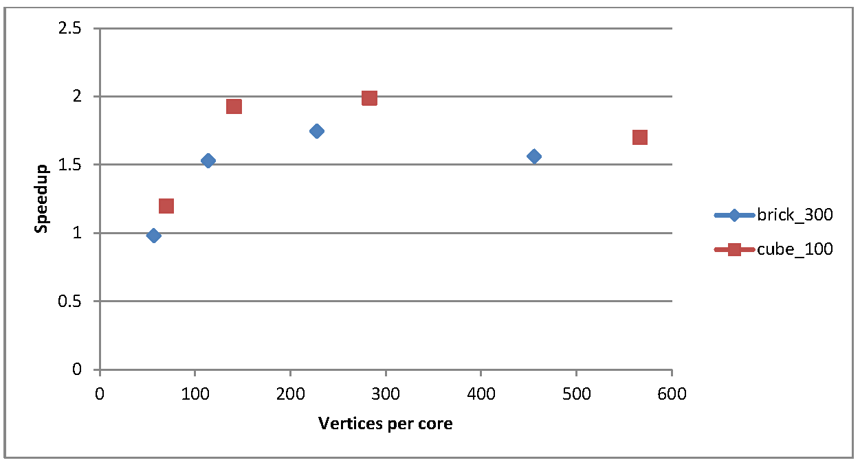
Figure 2: speedup as a function of vertices per core after data distribution
Now to consider the much larger test case, sphere. For this case, the initialisation is a larger proportion of the total runtime, approximately 3% for the sequential version. Also, due to time constraints some of the benchmarking runs were only performed for one thousand timesteps rather than to full convergence (a single core run of this benchmark takes approximately 10 hours to converge). Thus Figure 3 shows the speedup at 1000 timesteps for two cases: the purely parallel calculation, and the combined total speedup including initialisation. Of course, as it was a limited timestep run the initialisation becomes even more significant, and in fact accounts for over half the execution time beyond four cores at 1000 timesteps. Clearly though, one can see that the speedup is much more pronounced for this large test case, hitting 5 times faster at 16 cores.
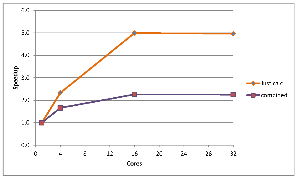
Figure 3: Speedup for sphere, for pure calculations and for calculations and initialisation combined, for 1000 timestep runs
The repartioning was also tested on this test case, but in this instance a full run to convergence was performed (which also gives an idea of how the intialisation affects the total speedup).
Table 2: Timings for sphere to full convergence
|
|
Serial |
16 cores |
Speedup |
16 cores
repartitioned |
Speedup |
|
Initialisation |
890 |
1359 |
|
1905 |
|
|
Calculation |
30366 |
6121 |
5.0 |
7278 |
4.2 |
|
Total |
31256 |
7480 |
4.2 |
9183 |
3.4 |
Table 2 shows the timings for the sphere test case for three runs: serial, 16 cores, and 16 cores using the repartitioning. Unfortunately the figures indicate that the repartitioning does not offer any performance improvement, and in fact slows the code down. The repartitioning increases the time spent in intialisation as expected but, it also increases the time spent doing the calculation. It is not clear what is the cause for this, unfortunately due to time constraints no further investigation was possible.
6 Further work
Further investigation into the repartitioning would be desirable, as it is not clear why it has been detrimental to the performance. Also, there is scope for both serial and parallel optimisations in the code: much of this project was spent trying to ensure that the code produced correct answers rather than in performance optimisation, and during this the author has spotted various opportunities for performance enhancement which unfortunately time constraints have prevented. For example, there are several pointwise vector divides in the core algorithm which could be refactored to multiplications, and some static vectors which are recalculated at every timestep unnecessarily. The initialisation could also be parallelised. These and other suggestions will be passed on to the code owners.
7 Summary
The key aims of this project were: to complete the parallelisation of the code started in the original project, with particular focus on the generation of the stiffness matrices; and to incorporate a mesh repartitioning algorithm into the code in order to enhance performance. This has been partially achieved: the code now works correctly in parallel, which it did not at the start of the project. Speedups of over four times faster have been seen for a large test case, which for this class of finite element problem is not unreasonable. The code also now has the capability to utilise repartitioning, although initial results suggest that this does not enhance performance.
The scientific goal of this project was to enable the investigation of large-scale simulations with increased system-size and precision which are currently not possible. These simulations will be of benefit to research into mineral- and palaeo-magnetism. This has been achieved, as the code can now be used to run large simulations, in parallel, taking advantage of the memory and compute power available on HECToR. In addition, the code makes use of the PETSc library, so should be portable to other systems.
8 Acknowledgements
This project was funded under the HECToR Distributed Computational Science and Engineering (CSE) Service operated by NAG Ltd. HECToR - A Research Councils UK High End Computing Service - is the UK’s national supercomputing service, managed by EPSRC on behalf of the participating Research Councils. Its mission is to support capability science and engineering in UK academia. The HECToR supercomputers are managed by UoE HPCx Ltd and the CSE Support Service is provided by NAG Ltd. http://www.hector.ac.uk
References
[1] The SUNDIALs library https://computation.llnl.gov/casc/sundials/main.html
[2] The Metis library http://glaros.dtc.umn.edu/gkhome/views/metis
[3] The PETSc library http://www.mcs.anl.gov/petsc/petsc-as/
[4] The Edikt project http://www.edikt.org.uk/edikt2/