 |
Ning Li
Numerical Algorithms Group (NAG)
Wilkinson House, Jordan Hill Road,
Oxford, OX2 8DR, UK
Date: February 28, 2011
This Distributed Computational Science and Engineering (dCSE) project is to modernise Incompact3D, a CFD application that performs Direct and Large-eddy Simulations (DNS/LES) of turbulent flows. This work is in collaboration with the Turbulence, Mixing and Flow Control group at Imperial College London, with Prof. Christos Vassilicos being the PI and Dr. Sylvain Laizet, the original code author, being the main academic collaborator. The main objective of this project is to rewrite Incompact3D's communication routines, in particular to update its domain decomposition strategy from 1D slab decomposition to 2D pencil decomposition, in order to improve its scalability on HECToR, and indeed, on any modern supercomputers.
The project was granted 16 months full-time effort for one person to work on a full-time basis, which translates to roughly 26 months effort on a 60% part-time basis. The project started in April 2009. At the very early stage of this project, it became apparent that many other applications could benefit from this work, in particular those CFD applications built on 3D Cartesian meshes using spatially implicit numerical schemes. As a result, a decision was made to pack the reusable software components into a library, called 2DECOMP&FFT, to facilitate the knowledge transfer from this project to a wider scientific community.
2DECOMP&FFT is a Fortran library to conduct two major tasks. At lower level it implements a 2D domain decomposition algorithm (also known as `pencil' or `drawer' decomposition) for applications based on 3D Cartesian data structures. At higher level it also provides a simple and efficient FFT interface to perform three-dimensional distributed FFTs. The library is optimised for large-scale computations on supercomputers and scales well to hundreds of thousands of processors. It relies on MPI but provides a user-friendly programming interface that hides communication details from application developers.
For Incompact3D, the introduction of the new decomposition strategy makes it scalable to 16384 cores on HECToR with high parallel efficiency. This has significantly improved the research group's productivity. The library development work also turns out to be an excellent idea. At the time of writing, one separate dCSE project is ongoing, using 2DECOMP&FFT to upgrade combustion code DSTAR. Several other projects are in the pipeline.
The rest of this report is organised as follows. In section 2, an overview of the 2D decomposition strategy is given. Section 3 briefly introduces the 2DECOMP&FFT package. Section 4 presents 2DECOMP&FFT's decomposition API. Section 5 reviews various software that can be used to compute Fast Fourier Transform in parallel on HECToR. Section 6 describes 2DECOMP&FFT's FFT API and its parallel performance is shown in Section 7. For modern multi-core supercomputers like HECToR, shared-memory programming becomes increasingly popular. A shared-memory implementation has been built in the foundation of 2DECOMP&FFT and is discussed in Section 8. Section 9 covers the numerical algorithms used by CFD application Incompact3D. In particular a spectral solver for the pressure Poisson's equation and its implementation is discussed. The section also covers the performance of the new Incompact3D code. Finally, conclusions and future works are summarised in Section 10.
There are two approaches to performing such computations on distributed-memory systems. One can either develop distributed algorithms (such as a parallel tridiagonal solver or a parallel FFT algorithm working on distributed data), or one can dynamically redistribute (transpose) data among processors in order to apply serial algorithms in local memory. The second approach is often preferred due to its simplicity: existing serial algorithms (hopefully already optimised for a single CPU) remain unchanged; porting serial code can be straight-forward as much of the original code logic still holds, and the only major addition is the data transposition procedures.
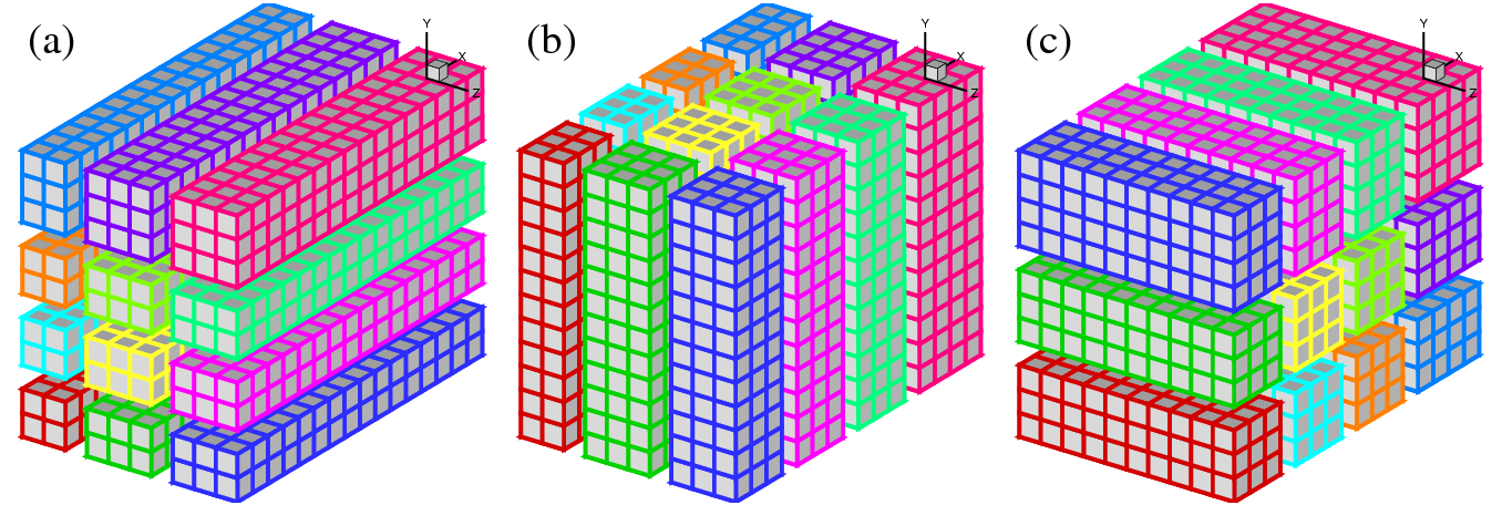
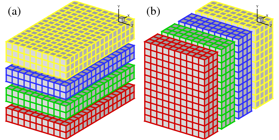
In early days of supercomputing, many applications implemented the above idea using 1D domain decomposition (also known as `slab' decomposition). In Fig.1, a 3D domain is arbitrarily chosen to be decomposed in Y and X directions. It can be seen that in state (a), any computations in the X-Z planes can be done in local memories while data along a Y mesh-line is distributed. When it is necessary to calculate along Y mesh-lines (say to evaluate Y-derivatives, or to perform 1D FFTs along Y), one can redistribute the data among processors to reach state (b), in which any computation in Y becomes `local'. If using standard MPI library, swapping between state (a) and (b) can be achieved using MPI_ALLTOALL(V) subroutine.
|
A 1D decomposition, while quite simple, has some limitations, especially for large-scale simulations. Given a cubic mesh of size N3 , one obvious constraint is that the maximum number of processors Nproc that can be used in a 1D decomposition is N as each slab has to contain at least one plane of data. For a cubic mesh with 1 billion points (which is very large but becomes increasingly common in CFD applications), the constraint is Nproc < = 1000 . This is a serious limitation as most supercomputers today have more than 10,000 cores and some have more than 100,0001. Large applications are also likely to hit the memory limit when each processor handles too much workload.
A 2D decomposition (also known as a `pencil' decomposition) is a natural extension to 1D decompositions. Fig.2 shows that the same 3D domain as in Fig.1 can be partitioned in two dimensions. From now on, states (a), (b) and (c) will be referred to as X-pencil, Y-pencil and Z-pencil arrangements, respectively. While a 1D decomposition algorithm swaps between two states, in a 2D decomposition one needs to traverse 3 different states using 4 global transpositions ( (a) = > (b) = > (c) = > (b) = > (a) ).
Again MPI_ALLTOALL(V) can be used to realise the transpositions. However it is significantly more complex than the 1D case. There are two separate communicator groups. For a Prow×Pcol processor grid: Prow groups of Pcol processors need to exchange data among themselves for (a) < = > (b) ; Pcol groups of Prow processors need to exchange data among themselves for (b) < = > (c) .
On one hand, the proper implementation of the communication routines can be quite tricky. For example the communications are very sensitive to the orientations of pencils and their associated memory patterns. The packing and unpacking of memory buffers for the MPI library must be handled with great care for efficiency. These software engineering topics are almost certainly irrelevant to the scientific researches conducted by the applications.
On the other hand, although the idea of 2D decomposition has long been established, its adoption in real applications was not essential until recently, when ordinary researchers can realistically expect to regularly use thousands of cores on major supercomputers, therefore hitting the limitation imposed by 1D decomposition. In fact, the author is aware of at least 10 applications within the UK CFD community only that require such upgrade sooner or later.
These motivated the author to create the 2DECOMP&FFT library - a general-purpose library that can be reused outside the scope of this project - to handle these technical issues properly and to hide most software-engineering details from application developers who can concentrate on their scientific studies.
The 2DECOMP&FFT library has a two-layer design - with a general-purpose 2D decomposition library at the foundation for data distribution, and an FFT interface built on the top to perform three-dimensional parallel FFTs. In fact, a number of numerical algorithms can be built on top of the 2D decomposition library. It is therefore appropriate to call 2DECOMP&FFT a software framework. For example, large-scale spectral code can be built using basis functions other than Fourier. (Depending on boundary conditions, a Jacobian or a Chebyshev basis function may be used.) It is also possible to build an elliptic PDE solver using this framework, as will be discussed in Section 9.
2DECOMP&FFT is written in standard Fortran. A Fortran 95 compatible compiler is required to build the library.2. The communication code is based on standard MPI. A flexible design of the FFT interface makes it possible to use third-party FFT libraries for the actual computation (with 2DECOMP&FFT handling the data distribution only). For these reasons, the library and applications built upon it can be easily ported to other hardware. In fact, the new Incompact3D code has already been ported on to several other platforms (including Cray, IBM and SGI) with minimum efforts.
On HECToR, a binary version of 2DECOMP&FFT has been installed at
/usr/local/packages/nag/2decomp_fft/1.0.237/
To evaluate it, one can start from one of the test applications provided in the samples directory. For example, to compile sample code test2d.f90, copy it to your work space and do
      export DECOMP2D_DIR=/usr/local/packages/nag/2decomp_fft/1.0.237/
      ftn -I$DECOMP2D_DIR/include test2d.f90 -L$DECOMP2D_DIR/lib -l2decomp
          -l2decomp_fft -o test2d.exe
Please note this PGI-built binary package is for test purpose only, supporting only single-precision calculations and using a generic FFT implementation. For performance and flexibility, please obtain the source package in order to have full access to the software options and build it with more efficient FFT engines, such as FFTW or ACML FFT.
As per the spirit of dCSE, the source code is freely available to HECToR users. Please contact the developer Dr Ning Li (ning.li@nag.co.uk) to obtain the source, discuss your potential applications and CSE supports that may be obtained. The software will become part of the Open Petascale Libraries (http://www.openpetascale.org/) and source code will be made available to all under a suitable open-source software license.
2DECOMP&FFT library functions are provided in several Fortran modules. A base module contains 2D decomposition information and data distribution routines. A separate FFT module provides three-dimensional distributed FFT functions. There are also other utility functions such as a MPI-IO module for proper parallel I/O. The decomposition library will be discussed in this section while the FFT interface will be covered later in Section 6.
This subsection explains the key public interfaces of the 2D decomposition library. After reading this section, users should be able to easily build applications using this domain decomposition strategy. The library interface is designed to be very simple. One can refer to the sample applications for a quick start.
First of all applications should include this Fortran module at the beginning:
use decomp_2d
The public interface of the library includes a set of global variables containing the decomposition information - how the global data is distributed - that applications require to define their data structures. All these global variables should be read-only after being initialised by:
call decomp_2d_init(nx,ny,nz,P_row,P_col)
where nx
, ny
and nz
are the size of 3D global data to be distributed over a 2D processor grid
Prow×Pcol
. Note that none of the dimensions need to be divisible by Prow
or Pcol
. However, choose the numbers smartly to avoid significant load-imbalance, which could lead to poor performance. Also note that the constraints here are:
ProwFollowing is the list of global variables that can be used in applications. Obviously these names should not be redefined in applications to avoid conflict.3 Also note that some variables contain duplicate or redundant information just to simplify the programming.
It is recommended that an applications define its major data structures using these global variables in its main program immediately after initialising the decomposition library. Using allocatable arrays is preferred but it is also possible to use static arrays in subroutines, as shown in the following examples:
      ! allocate a X-pencil array
      allocate(var(xsize(1), xsize(2), xsize(3)))
      ! allocate a Y-pencil array using global indices
      allocate(uy(ystart(1):yend(1), ystart(2):yend(2), &
                  ystart(3):yend(3)))
      ! define a Z-pencil work array in a subroutine
      real, dimension(zsize(1),zsize(2),zsize(3)) :: work1
The key element of the library is a set of communication routines that actually perform the data transpositions. As mentioned in Section 2, one needs to perform 4 global transpositions to go through all 3 pencil orientations. Correspondingly, the library provides 4 communication subroutines:
      call transpose_x_to_y(in, out)
      call transpose_y_to_z(in, out)
      call transpose_z_to_y(in, out)
      call transpose_y_to_x(in, out)
The input array in and output array out should have been defined for the correct pencils in the calling program.
Note that the library is written using Fortran's generic interface so different data types are supported without user intervention. That means in and out above can be either real arrays or complex arrays, the latter being useful for FFT-type of applications.
As seen, most of the communication details are packed within a black box and it is not necessary for application developers to understand the internal logic of these transposition routines. It is however noted that the communication routines are expensive, especially when running on large number of processors. So applications should try to minimize the number of calls to them by adjusting the algorithms in use, or even by duplicating some computations.
Finally, before exit, applications should clean up the memory by:
call decomp_2d_finalize
While the basic decomposition API is very user-friendly, there may be situations in which applications need to handle more complex data structures. One typical scenario in CFD applications is the use of staggered mesh which requires different storage for global quantities (cell-centred vs. cell-interface storage). Another example is when using real-to-complex FFTs, application needs to store both the real input (of global size nx*ny*nz) and the complex output (of smaller global size - such as (nx/2+1)*ny*nz - where roughly half the output is dropped due to conjugate symmetry).
Applications need to be able to distribute different data sets as 2D pencils. 2DECOMP&FFT provides a powerful and flexible programming interface to handle this:
      TYPE(DECOMP_INFO) :: decomp
      call decomp_info_init(mx, my, mz, decomp)
Here decomp
is an instance of Fortran derived data type DECOMP_INFO encapsulating the 2D decomposition information associated with one particular global size. The decomposition object can be initialised using the decomp_info_init routine. This object then can be passed to the communication routines defined in the basic interface as a third parameter. For example:
call transpose_x_to_y(in, out, decomp)
The third parameter is optional and can be safely ignored by users using the basic interface only. When it is in use, the global transposition will be applied to the associated global size instead of the default global size nx*ny*nz
.
Fast Fourier Transform (FFT) provides the basis of many scientific algorithms. There are hundreds of FFT software packages available. In this section, only those closely related to this project, especially those available on Cray systems are reviewed.
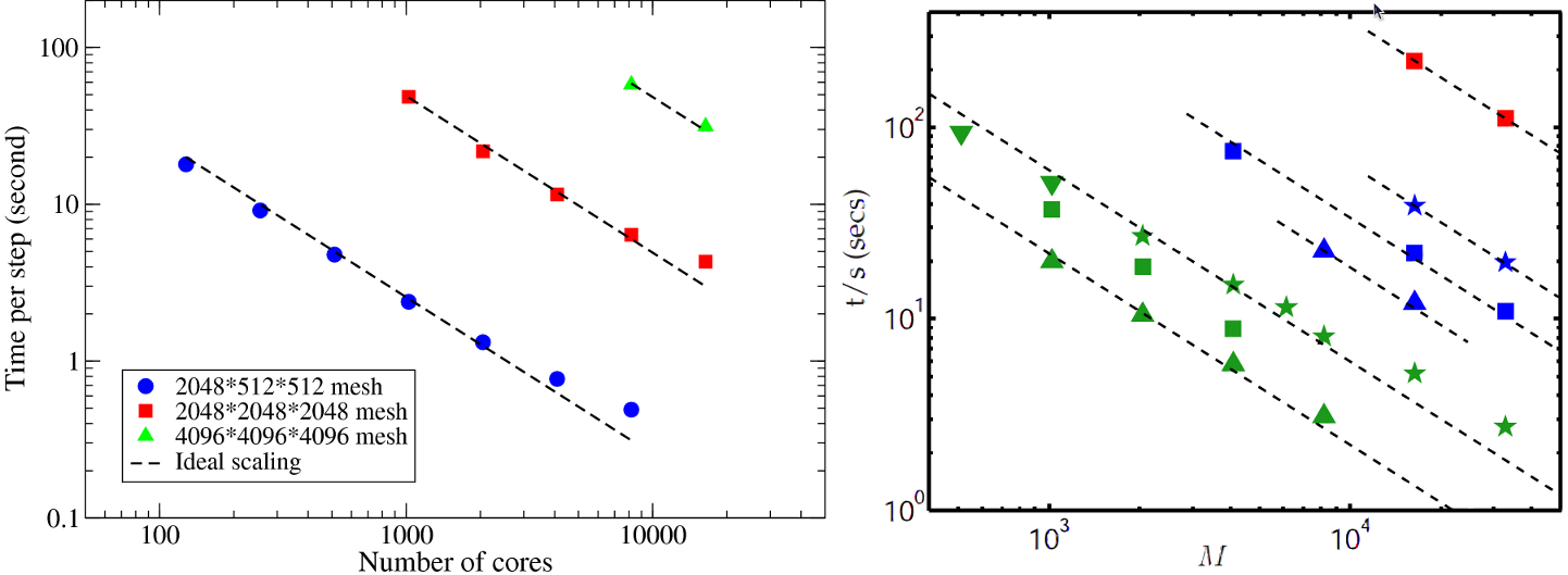
P3DFFT was actually ported onto HECToR at the early stage of this project. Fig. 3 shows its good scaling on the old phase 1 dual-core hardware. What motivated the author to develop a new and somewhat competing library are the following:
The distributed FFT interface only performs data management and communications. The actual computations of 1D FFTs are delegated to a 3rd-party FFT library, assuming it is already fully optimised to run on a single CPU core. Currently 2DECOMP&FFT users can select one of the 6 FFT engines at compile time as follows.
To use the FFT programming interface, first of all, one additional Fortran module has to be used.
use decomp_2d_fft
As mentioned earlier, the FFT interface is built on top of the 2D decomposition library, which, naturally, needs to be initialised first.
call decomp_2d_init(nx,ny,nz,P_row,P_col)
Then one needs to initialise the FFT interface by:
call decomp_2d_fft_init
The initialisation routine handles planing for the underlying FFT engine (if supported) and defines global data structures (such as temporary work spaces) for the computations. By default, it assumes that physical-space data is stored in X-pencil. The corresponding spectral-space data is stored in transposed Z-pencil format after the FFT. To give applications more flexibility, the library also supports the opposite direction, if an optional parameter is passed to the initialisation routine:
call decomp_2d_fft_init(PHYSICAL_IN_Z)
Physical-space data in Y-pencil is not an option as it would require additional expensive transpositions which does not make economical sense.
The main function this FFT package provides is to perform 3D FFTs where the distributed input data is stored in ordinary ijk-ordered 3D arrays across processors. For complex-to-complex (c2c) FFTs, the user interface is:
call decomp_2d_fft_3d(in, out, direction)
where direction can be either DECOMP_2D_FFT_FORWARD for forward transforms, or DECOMP_2D_FFT_BACKWARD for inverse transforms. The input array in and output array out are both complex and have to be either a X-pencil/Z-pencil combination or vice versa, depending on the direction of FFT and how the FFT interface is initialised (PHYSICAL_IN_X, the optional default, or PHYSICAL_IN_Z).
While the c2c interface is already in the simplest possible form, for many applications using real numbers only, the 3D FFT interface can be used in a more compact form:
call decomp_2d_fft_3d(in, out)
Here if in is a real array and out a complex array, then a forward FFT is implied. Similarly a backward FFT is computed if in is a complex array and out a real array.
When real input is involved, the corresponding complex output satisfies so-called `Hermitian redundancy' - i.e. some output values are complex conjugates of others. Taking advantage of this, FFT algorithms can normally compute r2c and c2r transforms twice as fast as c2c transforms while only using about half of the memory. Unfortunately, the price to pay is that application's data structures have to become slightly more complex. For a 3D real input data set of size nx×ny×nz , the complex output can be held in an array of size (nx/2 + 1)×ny×nz , with the first dimension being cut roughly in half4. Applications can either rely on the advanced interface described in Section 4.2, or use the following utility subroutine to distribute the complex output as 2D pencils:
call decomp_2d_fft_get_dims(start,end,size)
Here all three arguments are 1D array of three elements, returning to the caller the starting index, ending index and size of the sub-domain held by the current processor - information very similar to the start/end/size variables defined in the main decomposition library discussed earlier.
Please note that the complex output arrays obtained from X-pencil and Z-pencil input do not contain identical information. However, if `Hermitian redundancy' is taken into account, no physical information is lost and the real input can be fully recovered through the corresponding inverse FFT from either complex array.
Finally, to release the memory used by the FFT interface:
call decomp_2d_fft_finalize
It is possible to re-initialise the FFT interface in the same application at the later stage after it has been finalised, if this becomes necessary. To obtain first-hand experience on the FFT interface, users are advised to examine the sample FFT applications distributed with the library.
The performance of a distributed FFT library is determined by both the computation efficiency of the underlying 1D FFT algorithm and the communication efficiency of the data transposition algorithm. The following table shows the speed-up this library can achieve over the serial runs using FFTW's 3D FFT interface. The times reported (on HECToR phase 2a hardware) are for forward c2c transforms and all the transforms were planned using FFTW_ESTIMATE.
| Data size N3 | Serial FFTW | Parallel 2DECOMP&FFT | |||
| Planning | Execution | 16 cores | 64 cores | 256 cores | |
| 643 | 0.359 | 0.00509 | 0.00222 | - | - |
| 1283 | 1.98 | 0.0525 | 0.0223 | 0.00576 | 0.00397 |
| 2563 | 8.03 | 0.551 | 0.179 | 0.0505 | 0.0138 |
| 5123 | 37.5 | 5.38 | 1.74 | 0.536 | 0.249 |
| 10243 | - | - | - | 4.59 | 1.27 |
| 20483 | - | - | - | - | 17.9 |
It can be seen that due to the communication cost, the absolute speed-up over the serial library isn't great (only about 20-40 times on 256 cores). However, the parallel library does allow much larger problems to be computed quite efficiently. In particular, for smaller core count (16 and 64), each time the problem size is increased by 8 times, the computing time increases by 8-10 times, following the trend of the underlying serial library very well.
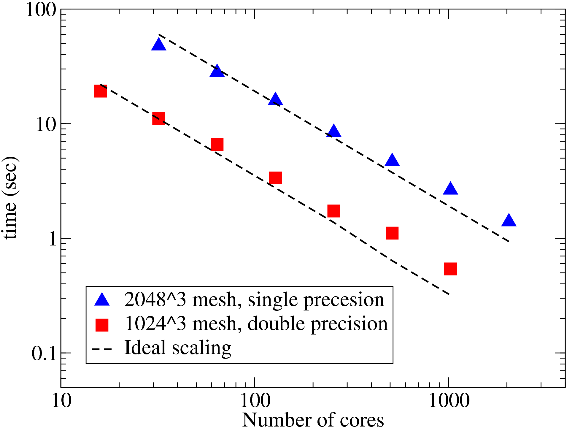
Large-scale parallel benchmarks of the FFT interface were performed on HECToR and Jaguar5, using problem size up to 81923 . The results presented in Fig. 4 are the time spent to compute a pair of forward and backward transforms on random signals. Both c2c and r2c/c2r transforms were tested. The underlying FFT engine is the ACML FFT (version 4.3). In all cases, the original signals were recovered to machine accuracy after the backward transforms - a good validation for the library. Up to 16384 cores were used on HECToR quad-core phase 2a system and each case was repeated 3 times and the fastest results were recorded. On Jaguar, the world No. 1 system at the time of the benchmark, a few very large tests were arranged using up to 131072 cores. Note that the runtime performance does vary a lot for such communication intensive applications, particularly on busy systems.
It can be seen that the FFT interface scales almost perfectly on HECToR for all the tests done. As expected, r2c/c2r transforms are twice as fast as c2c transforms. On Jaguar, the scaling is less good for larger core counts but the efficiency is still at a respectable 81% for the largest test. For a particular configuration - 40963 mesh on 16384 cores - the time spent on Jaguar is almost twice of that on HECToR. This is not unexpected. The test was ran on hardware with two 6-core chips. In order to achieve better load balance, the problem sizes need to have a factor of 6 which was not the case in these tests. Also the problem size 81923 , while quite large for real-world applications, is indeed too small when distributing over 105 cores.
The benchmark on the HECToR phase 2b system was also carried out. Due to the significant hardware architecture change, the scaling behaviour is very different. The results will be presented later in Section 8 where shared-memory programming is discussed.
The global transpositions and MPI_ALLTOALL type of communications are known to be very demanding for network bandwidth. So it is almost certain that large applications can run faster on under-populated nodes (see Fig. 10). This may also improve the computational efficiency due to improved memory bandwidth. Unfortunately this is rarely practical on most supercomputers where the resource charging is on per-node basis. Shared-memory programming, as will be discussed in Section 8, may improve the situation.
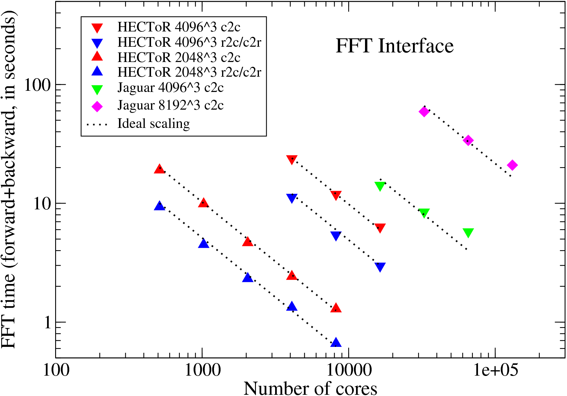
When using 2DECOMP&FFT, application users need to be aware that they have the freedom to choose the 2D processor grid Prow×Pcol . Depending on hardware, in particular the network layout, some processor-grid options deliver much better performance than others. Application users are highly recommended to study this issue before running large simulations.
Fig. 5 shows the performance of a test application using 256 MPI ranks on HECToR. It can be seen that in this particular test, Prow < < Pcol is the best possible combination for this hardware (the old Cray SeaStar2 interconnect). There are several technical reasons for such behaviour. First of all the hardware was equipped with quad-core processors (4-way SMP). When Prow is smaller than or equal to 4, half of the MPI_ALLTOALLV communications are done entirely within physical nodes which can be very fast. Second, as the communication library handles ijk-ordered arrays, small Prow (therefore larger nx/Prow , the inner-most loop count) tends to offer better cache efficiency for the computational parts of the code.
Please note that the behaviour reported in Fig. 5 is by no means representative. In fact the behaviour is also highly dependent on the time-varying system workload and the size and shape of the global mesh, among other factors. An auto-tuning algorithm is included in the library and can be switched on as follows:
call decomp_2d_init(nx,ny,nz,0,0)
When initialising the decomposition library, if a processor grid is specified as 0× 0
, an auto-tuning algorithm is used to determine the best processor grid at runtime. This, however, only takes into account the communication costs. Computation intensive code might benefit more from the cache efficiency factor. So application users are eventually responsible for selecting the best processor grid.
For ALLTOALL type of communication in which each MPI rank has to send/receive messages to/from all other MPI ranks, one can imagine that traffic from cores on the same physical node compete for their network interface. Even if the network bandwidth is sufficient, the performance is likely to be affected by network latency when too many small messages are passed with the system. One solution is to create shared send/recv buffers on each SMP node. Then only leaders of the nodes participate MPI_ALLTOALL(V), resulting in fewer but larger messages, hopefully improving the communication performance. The interconnects of supercomputers are often optimised for handling small amount of large messages.
This feature has been implemented within the communication library as a black box. It can be activated by users at compile time by using `-DSHM' flag. The shared-memory code uses the System V Inter-Process Communication (IPC) API which is widely supported on many variants of UNIX. Thanks for the contribution of several HECToR colleagues, 2DECOMP&FFT actually has two independent shared-memory implementations:
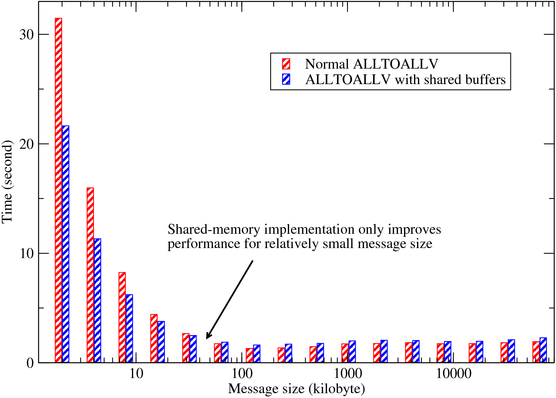
Fig. 6 demonstrates the typical benefit of shared-memory programming. The data was collected on HECToR phase 2a system from a series of simulations using 256 MPI ranks over a range of problem sizes. When the problem size is small (so is the message size), the communication routines were called more times so that the total amount of data moving within the system remains a constant. Fig. 6 shows that when the problem size is small, the overhead of setting up communications is very high and the shared-memory code can improve communication efficiency by up to 30%. As the problem size increases, the benefit of using shared-memory code becomes smaller. In fact for large message size (> 32Kb in this example), the shared-memory code is actually slower due to the extra memory copying operations required.
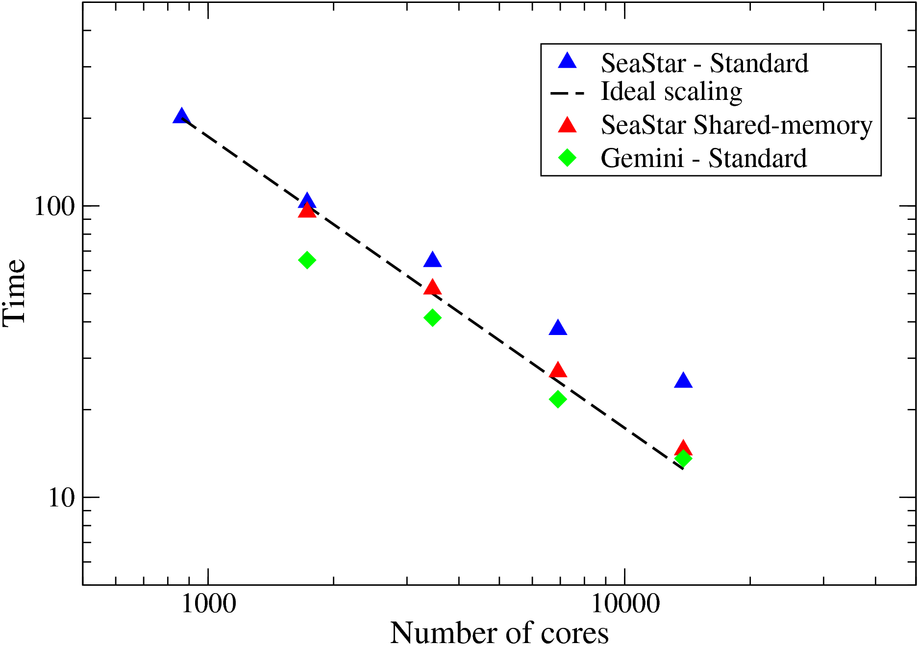
The HECToR upgrade to phase 2b presented a unique opportunity to show the benefit shared-memory programming can produce in real applications. The 24-core nodes were introduced to HECToR several months before the arrival of the new Gemini interconnect. During the transitional period, communication intensive applications could easily produce more network traffic than the old SeaStar interconnect could handle. Fig. 7 shows the benchmark of 2DECOMP&FFT's FFT interface using a problem size of 25923 . With the slow SeaStar interconnect, the scaling is very poor when using more than several thousands of cores. However, switching on the shared-memory code significantly improved the code performance (sometimes by more than 40%) and a parallel efficiency of more than 90% was observed through out the scale. The new Gemini interconnect offers significant improvement in terms of both network bandwidth and latency. As a result, significant performance gain is to be expected for communication intensive code. The FFT benchmark is almost twice as fast in some cases. However, the shared-memory code on Gemini (not shown in the figure) offers absolutely no benefit when the network is fast enough to handle all the messages efficiently. It actually slows down the application due to extra memory copying required to assemble/dissemble shared memory buffers.
After all the library development work, it finally comes to the point where the CFD application can be introduced. This section will first briefly cover the scientific background of the project, then discuss the numerical algorithms in use and the associated parallel-implementation strategy, and finally report of the parallel performance of the new code after the dCSE work.
This project concerns the development of a unique CFD application Incompact3D to make the best use of the recent unprecedented developments in HPC technology, and to improve our understanding of fluid turbulence.
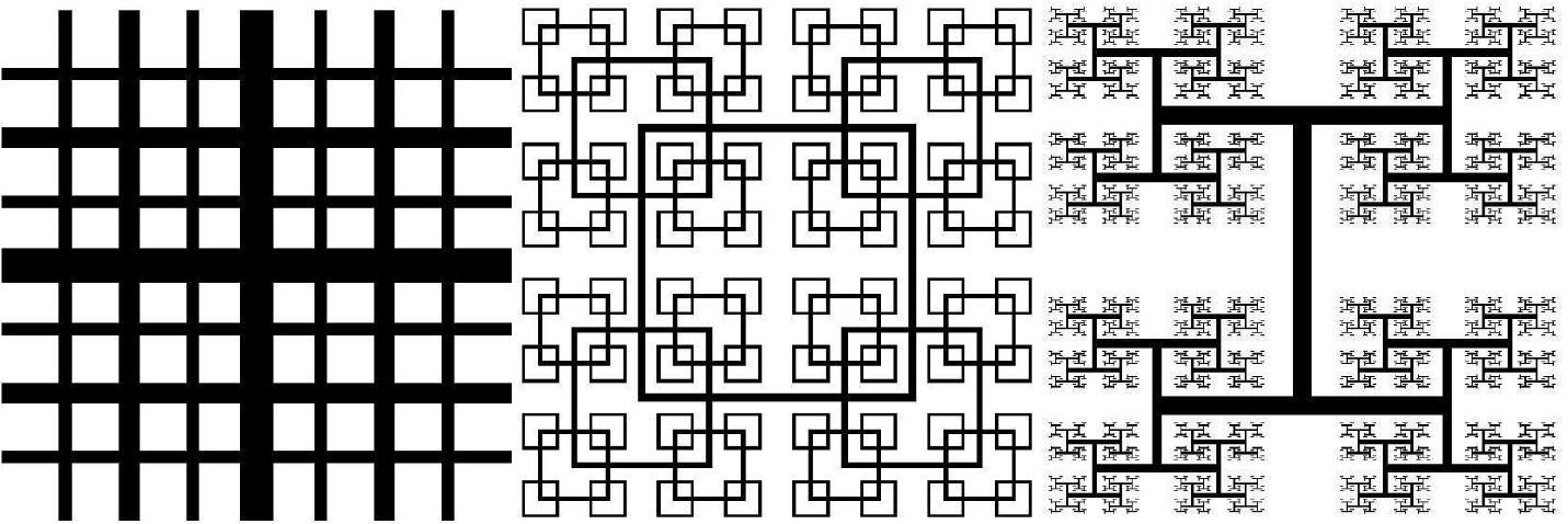
The academic partners at the Turbulence, Mixing and Flow Control group at Imperial College London have been working on cutting-edge energy problems for nearly a decade. One very recent example of their work is a new flow concept concerning turbulence generated by multiscale/fractal objects (as shown in Fig. 8). This class of new flow concepts is offering possibilities for brand-new flow solutions useful in industrial mixers, silent air-brakes, new ventilation and combustion devices. Many wind tunnel measurements have been performed successfully at Imperial College[10][15]. To complement these experimental results, high-resolution simulations of such multiscale flows are required in order to understand the underlying physics.
It can be seen that in order to resolve the turbulent eddies associated with the smallest scale, very large simulations are required. In fact, the number of mesh points required is often in the order of billions. This demands significant software development in order to properly use the supercomputing facilities available. The group was awarded 4 million HECToR AUs through an EPSRC grant and it also has access to HECToR resources via UK Turbulence Consortium. It is therefore important to produce highly scalable and efficient code to make good use of the resources.
Incompact3D is a CFD application solving the governing equations of fluid problems in incompressible form. When parallelising such applications, there are often two areas requiring major development efforts: the spatial discretisation and approximation of the Navier-Stokes equations; and the solving of the pressure Poisson's equation to enforce mass conservation. The complete coverage of Incompact3D's algorithms is published by Laizet & Lamballais[12]. This report will only highlight key areas that are relevant to code parallelisation.
Incompact3D uses a 6th order compact finite difference scheme to discretize the convective and diffusive terms of Navier-Stokes equations on a Cartesian mesh. The operators for evaluating spatial derivatives and doing spatial interpolations take an implicit form. For example, the first derivative on a collocated mesh can be calculated using:
 + b + b |
(1) |
There are various numerical algorithms solving the pressure Poisson's equations, broadly classified into two categories: iterative solvers and direct solvers. The Multigrid approach is often considered most efficient iterative method while FFT-based solvers are the most efficient direct methods.
There are actually two types of FFT-based approaches to solve Poisson's equations. The first type, sometimes referred to as matrix decomposition, uses Fourier's method to treat the finite difference discretisation of Poisson's equations. Using ordinary central differencing, a finite difference discretisation of a 3D Poisson's equation results in a linear system with seven diagonal lines. To solve the system quickly, one can apply Fourier analysis in one dimension, reducing the system to a number of pentadiagonal systems. Fourier analysis in a second dimension further reduces the problem to many tridiagonal systems which can be solved efficiently. The mathematical formulations of such method, in particular the proper treatment of non-periodic boundary conditions and the applications on different mesh configurations (staggered vs. collocated mesh), were established in 1970's[16][17] and a serial implementation is available in the form of open-source software FISHPACK[4]. This method actually fits in the 2DECOMP&FFT framework very well - one can apply 1D FFTs and a tridiagonal solver direction by direction in local memory, given that the data involved is properly redistributed using the transposition routines.
The Poisson solver adopted by Incompact3D is of a second type - a fully spectral treatment of the Poisson's equation, in order to directly take advantage of the 3D distributed FFT library developed. The algorithm involves the following steps:
The pre- and post-processing can be either local - meaning that operations can be done regardless of the parallel distribution of data, or global - meaning that calculations are only possible when data sets involved are all local in memory (i.e. the operations have to be done in a particular pencil-orientation). Fortunately, for the global case, whenever the data required is not available, the global transposition routines provided by the base library can be used to redistribute the data. A pair of forward and backward FFTs with 2D decomposition requires 4 global transpositions. Depending on the physical boundary conditions, the pre- and post-processing above may add up to 12 more global transpositions.
The old Incompact3D was parallelised using a 1D slab decomposition. This seriously limited its applications to large-scale simulations. For example, a typical simulation using a 2048*512*512 mesh can only use up to 512 cores. On HECToR phase 1 hardware, this translates to a runtime of 25 days (wall-clock time) or 50 12-hour sessions, excluding queueing time. Obviously at this rate it is impossible to conduct productive scientific studies.
The new Incompact3D has been completely rewritten using the 2DECOMP&FFT library, making it scalable to tens of thousands of cores on HECToR. To examine the performance of the new Incompact3D, several simulations were set up on meshes up to 40963 points and ran on HECToR using up to 16384 cores (72% of the full capacity of the phase 2a hardware). The results are shown in Fig. 9.
 |
It can be seen that the new code scales extremely well on HECToR. In comparison, the scaling results of P. K. Yeung's spectral DNS code[9] based on P3DFFT library are reproduced here. What is directly comparable is the data set taken from supercomputer Franklin (was also a Cray XT4) shown as green triangles, exhibiting very similar scaling behaviour.
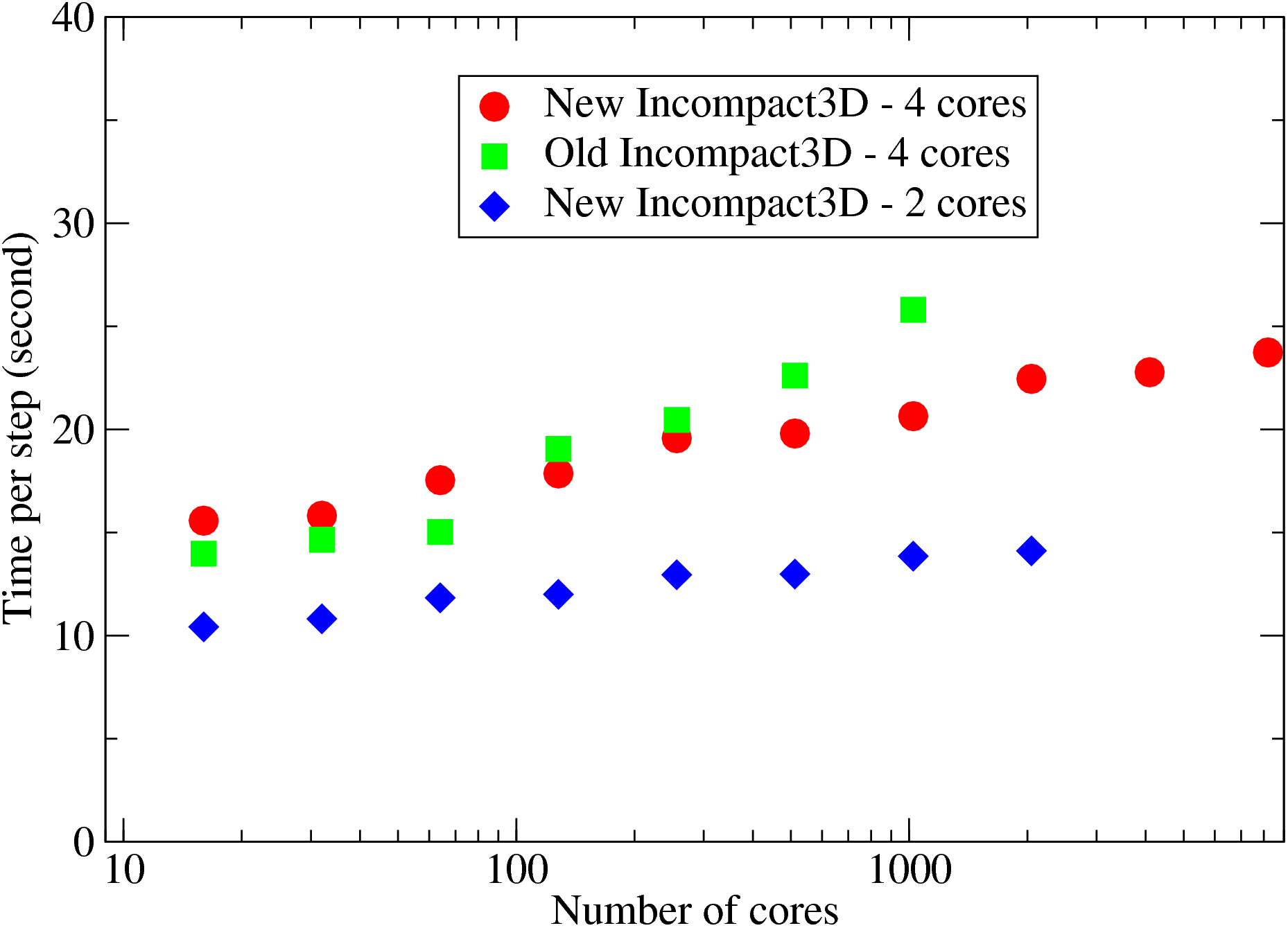
Fig. 10 shows the weak scaling of Incompact3D at a workload of 4191304 mesh points per MPI rank. A performance comparison between the old and the new code on HECToR phase 2a hardware is given. The old Incompact3D, implemented using a 1D slab decomposition, is faster on smaller core counts. But the new Incompact3D outperforms the old code for larger cases, partly because the communications are only among subsets of MPI ranks which is more efficient.
In addition to the moderate performance gain (about 20% at 1024 cores), note that the constraint applied by the 1D decomposition to the old code (1024 cores in this test) does not apply to the new code. This improved scalability allows the research group to conduct much larger simulations within much shorter period of times, producing scientific results quickly.
Fig. 10 also shows that when using only 2 cores per quad-core node, the code is consistently 30% faster due to improved memory and network bandwidth. This suggests that introducing another level of parallelism at node level, possibly through the use of OpenMP for the computational part of the job, may further improve the code performance.
While working on this project, several objectives in the original proposal were dropped, including the planned work on a vector version of Incompact3D to produce a hybrid OpenMP/MPI code.
Shortly after the approval of the Incompact3D dCSE, a message from Cray advised that "there is a restriction on the X2 regarding hybrid OpenMP/MPI codes. Basically, OpenMP within MPI (or CAF or UPC) is not supported for multi-node applications. OpenMP should only be used for single-node applications, and MPI, CAF or UPC should be used for multi-node applications." This made the proposed work not so attractive. Subsequently a decision was made to introduce shared-memory code (as discussion in Section 8), which addresses the same technical problem from a different perspective.
According to Dr Laizet, "the vector version of Incompact3D will no longer be used for research purposes, except maybe for student projects." The planned use of X2 for post-processing (because of its large memory) was also dropped as a MPI code for the post-processing is now available (also built using 2DECOMP&FFT) and is running on the XE6 system.
Through this dedicated software-development project, the CFD application Incompact3D has been transformed into a modern, highly portable and highly scalable software package. Extremely good parallel performance has been demonstrated on HECToR and indeed several other supercomputing sites. This enables the academic partners to conduct very large-scale cutting-edge turbulence simulations.
One major contribution of this project is the creation of the 2DECOMP&FFT package, which encapsulates a general-purpose 2D decomposition library and a distributed FFT interface. This package will benefit many scientific applications undergoing similar upgrade. Currently, supported by dCSE, several other applications are being (or to be) updated using 2DECOMP&FFT, including a combustion code (DSTAR), a compressible DNS code (Compact3D) and an ocean modelling code.
In the future, it is worthwhile to introduce additional features to 2DECOMP&FFT in order to provide better application support, including:
The CFD code Incompact3D may benefit from further developments in the following areas:
Finally, additional information regarding the 2DECOMP&FFT library can be found in a Cray User Group paper[14]. And parallel performance of Incompact3D on other supercomputing sites are reported in a journal paper[13].
This project was funded under the HECToR Distributed Computational Science and Engineering (CSE) Service operated by NAG Ltd. HECToR - A Research Councils UK High End Computing Service - is the UK's national supercomputing service, managed by EPSRC on behalf of the participating Research Councils. Its mission is to support capability science and engineering in UK academia. The HECToR supercomputers are managed by UoE HPCx Ltd and the CSE Support Service is provided by NAG Ltd. http://www.hector.ac.uk
This document was generated using the LaTeX2HTML translator Version 2008 (1.71)
Copyright © 1993, 1994, 1995, 1996,
Nikos Drakos,
Computer Based Learning Unit, University of Leeds.
Copyright © 1997, 1998, 1999,
Ross Moore,
Mathematics Department, Macquarie University, Sydney.
The command line arguments were:
latex2html -split 0 -no-navigation -show_section_numbers -html_version 3.2,math -no-math -local_icons -antialias FinalReport
The translation was initiated by Ning Li on 2011-02-28