Abstract
The intrinsic time-scale of correlated electron motion in matter is the attosecond time-scale (1 attosecond = 10-18s) and just as femtosecond (1 femtosecond = 10-15s) laser technology offers us the means of accessing real-time nuclear dynamics, attosecond light pulse technology now promises us the revolutionary ability to measure and control the correlated motion of electrons in atomic systems on their own temporal scale. Recent ground-breaking ultrafast measurements demonstrate that a bottleneck in our understanding of correlated electron dynamics in atoms and molecules is the current state of theory. Correlated electron motion by its very definition is a quantum many-body process and so theoretical methods must go beyond the widely used single-particle picture so far employed to good effect to describe ultrafast single electron processes. Currently, the most sophisticated method that goes beyond the single particle model is that underlying the HELIUM code. Inspired by the success of HELIUM at describing the correlated motion of electrons within two-electron systems, the purpose of this dCSE project is to extend the capability of HELIUM to allow it to accurately describe the correlated electron dynamics occurring within complex atoms exposed to intense short-pulse light. This paper describes the underlying numerical methods and algorithms implemented to extend HELIUM into a powerful new Fortran 90/MPI code called RMT (R-Matrix incorporating Time) which is unique in its capability to describe the many-electron response of a general atom to intense short-pulse laser light. Illustrative results for single ionization of neon exposed to a combination of sub-femtosecond XUV and 800 nm Ti:sapphire laser light fields, along with a discussion of the performance of the new RMT code on HECToR, are included.
Over the past 10 years there has developed a crucial need to solve directly and accurately the Time-Dependent Schrödinger Equation (TDSE) describing the detailed response of many-electron atoms and molecules to short, intense pulses of light. Such calculations are vital to get the best out of Attosecond Science [1, 2] (1 atto-second (atto-s) is 10-18 seconds), the revolutionary goal of which is to track and control the correlated motion of electrons within matter on their own temporal scale. The advent of Attosecond Science is bringing about a revolution in both laser and electron collision physics. Experiments on the Attosecond Time-Scale (ATS) are in progress in leading laboratories in the UK [3, 4]; in wider Europe [5, 6, 7]; in North America [8, 9, 10, 11]; in China [12] and in Japan [13, 14]. It is expected that near-future advances in Attosecond Light Pulse (ALP) technology [2] will have profound implications for fields as diverse as bioenergetics [15], molecular electronics [16] and even the treatment of cancer [17].
Many of the technological breakthroughs in Attosecond Science over the last decade have come about as a result of advances in theory [18] which now allow for a sound qualitative understanding of the Single Active Electron (SAE) response of an atom or molecule to intense femtosecond (1 femto-second (fs) is 10-15 seconds) laser pulses at short and long wavelengths. Indeed, in the long wavelength regime, advances in Ti:Sapphire laser technology [19] combined with an improved understanding of SAE phenomena such as High Harmonic Generation (HHG) [20] have resulted in the recent generation of extreme ultraviolet (XUV) light pulses that last a mere ~ 100 attoseconds in duration [21].
While SAE-based theories have been employed to good effect over the last decade, ALP technology is now demonstrating the revolutionary potential to induce and track ultra-fast many-electron dynamics within atoms and molecules [5, 7]. There is therefore huge importance in the development of tractable methods that are able to treat the correlated motion of electrons in complex atoms and molecules exposed to intense (ultra)short light pulses. Currently, the most sophisticated code for describing correlated electron dynamics within an atomic system is the HELIUM code [24, 25]. HELIUM is a pioneering code in the area of Attosecond Science. Not only has it made possible important scientific discovery (afterwards borne out by laboratory experiment) [25] but it has, in doing so, explored the feasibility of propagating accurate solutions of a multi-dimensional TDSE. The code is specifically constructed to describe both single- and double-electron ionization of a two-electron atom or ion exposed to intense laser light. The code’s continuing success undoubtedly lies in the fact that, from the start, it was designed around MPP architectures [24] (recognized as being absolutely essential to progress in this area of research). The method kernel to the code is a high-order Arnoldi time-propagator [22, 23] combined with Finite Difference (FD) grid methods. By choosing an appropriate distribution over processors HELIUM involves only nearest neighbour communications and this has enabled it to scale highly effectively to more than 16,000 cores on HECToR.
It is this established efficiency, along with the experimental interest in strongly time-dependent atomic and molecular systems, that has inspired the designers of HELIUM to exploit its underlying numerical methods to treat complex many-electron atoms exposed to intense (ultra)short light pulses. In particular, the underlying FD technology of the HELIUM code appears to be well suited for the accurate and efficient description of one or two electrons ejected from a many-electron atom or molecule during the single or double ionization process. With this capability in mind, the designers of the HELIUM code have recently demonstrated the potential to carry over the FD technology of HELIUM into an accurate description of a general many-electron atom exposed to intense light pulses. This carry over has been shown to be possible by invoking the powerful division-of-space concept [26], central to the highly successful R-matrix theory of atomic and molecular processes [27]. The division-of-space concept, whereby the position space occupied by the atomic electrons is divided into two separate regions, not only makes possible the integration of FD technology into the description of the ultrafast ionization of many-electron atoms, but also allows an efficient way of limiting the many-electron representation of an atom to the only spatial region where it is absolutely necessary, i.e., a small region close to the nucleus. In this finite region it has been well-established that the R-matrix basis set functions offer an accurate and tractable means of representing the many-electron wave function [27]. Indeed, the combination of the R-matrix basis set with FD grid techniques brought together with the powerful Arnoldi propagator of the HELIUM code provides the potential to efficiently and accurately describe the full response of a many-electron atomic system to intense (ultra)short pulse light which has so far proven beyond the capability of all existing theoretical methods.
With this goal in mind, in early 2009 a five-year EPSRC Software Development Grant (the UK-RAMP Project) was awarded to four collaborating institutions: Queen’s University Belfast (QUB), University College London (UCL), the Open University and STFC CSE, to build upon expertise in all the various areas of ab initio theoretical electron- atom and molecule scattering and both time-independent and time-dependent laser-atom (molecule) interactions. A major strand of the UK-RAMP Project is the carry-over of HELIUM code technology to enable the accurate description of the full response of atoms and molecules to intense (ultra)short laser pulses. The first major and vital algorithmic advance required in the pursuit of this goal is the construction of an ab initio code that combines HELIUM code and R-matrix technology to describe the single-electron ionization response of a general many-electron atom exposed to intense (ultra)short light pulses.
The purpose of this dCSE project is to construct a unique application code that will allow for the accurate and efficient description of the single ionization response of a general many-electron atom exposed to an intense (ultra)short laser light pulse. This project therefore forms the first vital advance in the pursuit of codes that are capable of describing the multiple ionization of atoms as well as the single ionization of molecules exposed to intense light pulses as set out in the UK-RAMP Project. As a means of making this advance, the project significantly extends on the recent work carried out on interfacing FD methods with basis set methods for the description of the one-electron hydrogen atom [26]. In extending the method into one that can accurately and efficiently describe a general many-electron atom exposed to strong laser fields, three main tasks needed to be accomplished (over a 24 month period) which all required, as a starting point, significant serial code construction:
All of the tasks were completed within the specified time-frames.
This dCSE project has resulted in the construction of a unique application code, now known as the RMT code. The RMT code is a general-purpose ab initio computer code for accurately describing the many-electron response leading to single ionization of many-electron atoms and atomic ions exposed to intense laser light pulses. The ab initio nature of the code allows for not only the description and understanding of future experimental measurements, but will also enable the prediction of physical phenomena occurring in intense laser-atom interactions and consequently allow for scientific discovery that will point the way for future experimental investigations at laser labs and large scale facilities over the next decade, at least.
One of the unique features of the RMT code is that it has been designed specifically to be applicable to atoms exposed to wavelengths ranging right across the light spectrum, from the extreme ultraviolet (XUV) photon frequencies being produced at 4th Generation light sources such as FLASH, the future European XFEL facility and the LCLS in the USA, to the infrared (IR) frequencies being produced at Ti:sapphire-based laser labs throughout the UK (e.g., Artemis at the STFC’s Central Laser Facility) and wider Europe (e.g.,‘Laserlab-Europe’). Not only does the RMT code have flexibility over wavelength, but because of its genuinely time-dependent nature it also has the flexibility to describe the response of atomic systems to both short- and long-duration light pulses. Moreover, because of the explicit representation of the light field, the code will also be able to support the wide-range of experiments investigating the effects of temporal pulse-shaping on the response of atoms to laser light, an important step towards future control mechanisms in fields such as photochemistry and molecular electronics.
The ability of the RMT code to describe the dynamics of general many-electron atoms on the attosecond time scale will also be of immense benefit to all UK research groups developing and applying Attosecond Technology (STFC’s CLF, Imperial College London). The near-future promise of high-intensity attosecond light pulses holds out the prospect for the real-time observation and control of charge transfer in molecular systems which is expected to have a strong impact on the future of molecular electronics [15] and possibly cancer research [17]. While the RMT code described here will be capable of providing deep insight into the dynamics of electrons in many-electron atoms exposed to ultrashort pulses, the exciting and genuine potential to adapt the method to describe many-electron dynamics within molecular systems will rely heavily on the advances that were made during this project.
As a necessity, the starting point for describing the ultra-fast dynamics of electrons in an atom exposed to an intense (ultra)short light pulse is the Time-dependent Schrödinger Equation (TDSE).
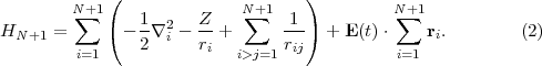
Neglecting relativistic effects, the behaviour of the N+1 electron atomic system in the presence of the laser field is governed by the TDSE
where the Hamiltonian is We have taken the origin of the coordinates to be in the nucleus, which we assume has infinite mass. We have rij = |ri - rj| where ri and rj are the vector coordinates of the ith and jth electrons and we have written XN+1 ≡ x1,x2,...,xN+1 where xi ≡ riσi. Z indicates the nuclear charge and E(t) is the time-dependent light field.
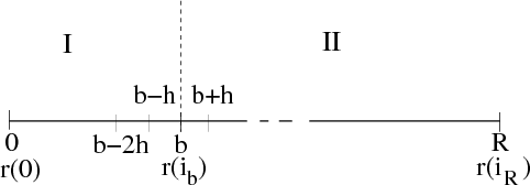
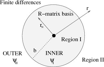
In the R-matrix method [27] the position space occupied by the electrons is divided into two regions: An inner region (region I) surrounding the nucleus where a many-electron wave function is constructed and many-electron atom-laser Hamiltonian matrix elements are calculated explicitly, and an outer region (region II), chosen such that only one electron (or at most two) is present and the electron there, besides experiencing the laser field directly, is aware of the remainder of the atomic system only via long-range multi-pole interactions. Traditionally, R-matrix theory is a theory where time is not explicitly involved in the study of the collision or photoionisation processes.
Figure 1 displays the division of many-electron position space which underlies R-matrix theory. In region I the time-dependent wavefunction is expanded over the R-matrix eigenstates of the field-free Hamiltonian. Region I is defined by all N + 1 electrons of the system having a radial co-ordinate rq ≤ b, q = 1,...,N + 1. Region II is defined by N electrons having a radial coordinate rq ≤ b, q = 1,...,N and one electron having its radial coordinate rN+1 > b. In region II the time-dependent wavefunction is represented over a finite-difference grid by its values at equidistant grid points rN+1(i) = ih,i = ib,ib + 1,...,iR.
Much of the power of the division-of-space concept is derived from limiting the many-electron representation of the atom to only the spatial region where it is absolutely necessary, i.e., region I, close to the nucleus of the atom. This means that the number of electrons in region II is limited to just one and hence the TDSE in region II is, for each state of the residual-ion, reduced in dimensionality to at most three, thus simplifying the computational problem considerably.
In region II, the time-dependent N+1 electron wave function can therefore be
expanded as Ψ(XN+1,t) = ∑
pnpΦp Fp(r,t), where the Fp functions are
single-electron functions describing the radial motion of the ejected electron
(in the pth-channel), and where the radial variable of the (N + 1)-th
electron is denoted as rN+1 = r. The Φp are channel functions formed by
coupling the target states of the residual ionic system Φp(XN ) with angular
and spin parts of the ejected electron wave function. Note that the time
dependence of the wavefunction is contained within the radial functions
Fp(r,t).
Fp(r,t), where the Fp functions are
single-electron functions describing the radial motion of the ejected electron
(in the pth-channel), and where the radial variable of the (N + 1)-th
electron is denoted as rN+1 = r. The Φp are channel functions formed by
coupling the target states of the residual ionic system Φp(XN ) with angular
and spin parts of the ejected electron wave function. Note that the time
dependence of the wavefunction is contained within the radial functions
Fp(r,t).
By projecting the known target functions Φp onto the TDSE and integrating over all spatial variables except the radial coordinate of the ejected electron, the following set of coupled homogeneous partial differential equations (PDEs) for the radial channel functions Fp(r,t) is obtained:
Eq.(3) is the evolution equation for the wave function in region II. In eq.(3), WE is referred to as the long range potential in the R-matrix literature and arises from the electron-electron and electron-nuclear potential terms in the Hamiltonian. WD arises from the interaction of the light field with the residual N-electron ion. The WP potential arises from the interaction of the light field with the ejected electron. Hti is the time-independent part of the Hamiltonian in region II.
This section describes a stand-alone code, TD-OUTER, that was constructed to solve eq.(3).
Software requirements:
Design strategy:
The TD-OUTER code was constructed on top of a well-tested one-electron version of the HELIUM code known as HYDRO. The HYDRO program uses the highly accurate and efficient Arnoldi propagator and FD techniques of HELIUM to propagate a single electron wave function forward in time. HYDRO has been written in Fortran 90 and has been parallelized using a similar strategy to that implemented in HELIUM using the Message Passing Interface (MPI). Since TD-OUTER describes the ejected electron in the presence of a many-electron atom it requires many-electron atomic structure data to construct the WE,WD and WP potentials appearing eq. (3). This data is calculated using the RMATRX2 suite of programs [28] which writes the atomic data to two files, H and d. All modifications to the HYDRO program at this stage of implementation were made using the single core version of the HYDRO program.
Definition of tasks:
In order to construct the TD-OUTER program two modifications to HYDRO were required:
HYDRO was designed to solve the single-electron TDSE using pure FD techniques and therefore it operates over the spatial domain 0 ≤ r ≤ R. The TD-OUTER program is required to solve an effective one-electron TDSE and is also to be interfaced with the basis set techniques (used over the domain 0 ≤ r ≤ b) which underly the TD-RA program. Therefore, a new FD grid needed to be laid so that TD-OUTER operates over the domain, b ≤ r ≤ R, i.e., from the R-matrix boundary outwards.
HYDRO was designed to solve the TDSE for the hydrogen atom and is therefore limited to describing a single state of a residual ion (which is the case for hydrogen where only a bare structureless proton is left behind by the ionizing electron). TD-OUTER is designed to solve an effective one-electron TDSE, where due to the many-electron nature of region I, the ejected electron is coupled to multiple residual ion states via long-range multipole potentials (WE(r) in eq.(3)). The ejected electron can couple to the residual ion states in multiple ways depending on the angular momentum of the ejected electron and the symmetry of the residual ion state, giving rise to the multiple channel functions Fp(r,t) of eq.(3). Moreover, these channels are coupled to each other via the time-dependent WD(t) and WP (r,t) potentials. All three of the potential terms in the eq.(3) needed to be coded into TD-OUTER.
|
Software implementation phase:
The FD grid was defined as a 1-dimensional (1D) grid representing the radial variable r of the ejected electron. The grid was laid out, as shown in figure 2, so that grid points lie at the two boundaries, r = b and r = R. Since TD-OUTER is required to compute the radial wave function flux pertaining to multiple states of the residual ion, the F vector as defined in HYDRO had its length increased to account for the extra channels formed by the multiple residual ion states.
The Hti operator in eq.(3) contains the second derivate operator,
 which is recast in a 5-point FD representation. However, the
5-point FD rule when applied to the Fp functions at the first grid
point, i=ib, requires information on the value of the Fp functions
at points i=ib-1 and i=ib-2 which lie inside region I, i.e., outside
the domain, b ≤ r ≤ R. This can be appreciated if one considers
the 5-point rule for calculating
which is recast in a 5-point FD representation. However, the
5-point FD rule when applied to the Fp functions at the first grid
point, i=ib, requires information on the value of the Fp functions
at points i=ib-1 and i=ib-2 which lie inside region I, i.e., outside
the domain, b ≤ r ≤ R. This can be appreciated if one considers
the 5-point rule for calculating  Fp at the left boundary r = b:
Test phase:
To test TD-OUTER, region I was made negligible in size by setting b = h. The points i=ib-1 and i=ib-2 then correspond to radial distances r = 0 and r = -h respectively. This FD grid is the same as that used in HYDRO and therefore similar boundary conditions as are used in HYDRO could be used in TD-OUTER to determine values of Fp at i=ib-1 and i=ib-2. The output from TD-OUTER was compared with that from HYDRO and was shown to match exactly, thus verifying the accuracy of the TD-OUTER code at this stage of construction.
Each residual ion state gives rise to a collection of channel functions, Fp, in region II which are coupled via the WE, WD and WP potentials.
WE(r): The space-dependent WE(r) potential is constructed using the long-range multipole coefficients calculated using the RMATRX2 suite of programs [28]. These coefficients are read into TD-OUTER from the H file written by RMATRX2.
WD(t): The time-dependent WD(t) potential is constructed using the dipole transition elements between the eigenstates of the residual ion which are calculated using the RMATRX2 programs. These matrix elements are read into TD-OUTER from the d file written by RMATRX2.
WP(r,t): The time- and space-dependent WP (r,t) potential is coded using angular algebra. It takes into account the symmetries of the residual ion states and of the ejected electron, read from the H file written by RMATRX2.
Test phase:
Testing at this stage was not feasible as it relies on the interfacing of TD-OUTER with TD-RA.
In region I, the time-dependent N+1 electron wave function Ψ(XN+1,t) is
represented over an R-matrix eigenbasis ψk(XN+1) as Ψ(XN+1,t) =
∑
kCk(t)ψk(XN+1) where rN+1 ≤ b and where Ck(t) are time-dependent
coefficients. The TDSE in the inner region is given by eq.(1). However, in region
I, the Hamiltonian HN+1 is not Hermitian owing to the presence of the
kinetic energy - ∇i2 term in eq.(2) and the finite value of the wave
function on the inner-region boundary. Consequently a Bloch operator
∇i2 term in eq.(2) and the finite value of the wave
function on the inner-region boundary. Consequently a Bloch operator
 N+1 =
N+1 =  ∑
i=1N+1δ(ri -b)
∑
i=1N+1δ(ri -b) is introduced which is such that HN+1 + N+1 is
Hermitian in region I. The TDSE in region I may then be written as
is introduced which is such that HN+1 + N+1 is
Hermitian in region I. The TDSE in region I may then be written as
where ΨI(XN+1,t) is the wave function defined over region I in figure 1. By projecting eq. (5) onto the eigenstates ψk(XN+1) we obtain the evolution equations for the time-dependent coefficients Ck(t):
where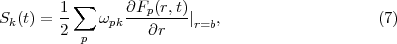
where


At this point it should be emphasized that eq.(6) is fundamental to the RMT method in two ways. Firstly, the inhomogeneous Sk term on the right-hand-side compensates for the Bloch term introduced to make HI Hermitian. Note that it makes a contribution only at r = b and brings into play there Ψ(XN+1,t), a wave function form which has been defined throughout both regions. This term is central to any time propagation scheme in region I because it connects the wave function form ΨI(XN+1,t), which is many-electron in nature, with a wave function form that, at r = b, represents a single electron and which, numerically, is obtained from region II. Secondly, eq.(6) allows for two different numerical methods to be brought together, one (basis set) most appropriate to the many-electron finite region I and the other (finite difference), most appropriate to the one-electron region II. In this way eq.(6) is fundamental to future plans to adapt the method to many-electron molecules.
Software requirements:
Design strategy:
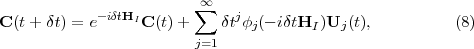
Eq.(6) takes the form of an inhomogeneous TDSE which arises in many areas of quantum dynamics. However, it is only recently that attempts have been made at using high-order explicit methods to solve equations of the type given by eq.(6). One such high-order propagator can be devised by approximating the formal solution explicitly by a Taylor expansion [32]. This is the method used for the single-electron implementation of the current method [26]. The approach taken in TD-RA is to compute the values of the Ck(t + δt) coefficients in eq.(8) using an adapted “inhomogeneous” Arnoldi method that in many ways resembles the standard Arnoldi method used for solving the homogeneous TDSE. The full implementation of the adapted Arnoldi algorithm will be described later in section 2.7. In this section a method is first implemented which focuses on propagating the Ck coefficients without the driving inhomogeneous terms that will be calculated in region II. In this way, the level of accuracy of the standard homogeneous Arnoldi method combined with the R-matrix basis set technology is first established.
Definition of tasks:
The construction of the TD-RA program requires the implementation of a single task:
Unlike the TD-OUTER code, the TD-RA program needed to be written from scratch. The first stage in developing TD-RA was to construct the many-electron time-dependent Hamiltonian whose matrix elements are calculated by the RMATRX2 codes. The second stage was to code the standard Arnoldi method to time-propagate the many-electron wave function. Once constructed, the time-dependent Hamiltonian is used to time-propagate the many-electron wave function using the standard Arnoldi method.
Implementation phase:
The ‘starter’ data written to file by RMATRX2 codes is needed to construct the Hamiltonian, HI . The matrix, HI, has a block-tridiagonal structure, with the diagonal blocks containing the field-free Hamiltonian for each symmetry of the many-electron atom (where a symmetry is defined in terms of the total angular momentum, L, the total spin, S, and the total parity, π, of the N+1 electron states). The eigenenergies, Ekk′, of the atom making up these diagonal blocks are read from the H file written by RMATRX2. The off-diagonal blocks contain the dipole couplings between the different angular momenta. The dipole matrix elements, Dkk′, making up these off-diagonal blocks are read from the d file, also written by the RMATRX2 programs.
As a starting point to solving eq.(8) via an Arnoldi-based method, the second term on the right-hand-side of eq. (8) was set to zero to neglect the inhomogeneous terms and to effectively constrain the laser-atom problem purely to region I. This poses no problem so long as region I is set large enough to fully contain the wave function throughout the propagation. This allowed the coding of the Arnoldi algorithm propagating the Ck from t to t+δt to be extensively tested in the absence of region II.
An Arnoldi/Lanczos algorithm was coded to propagate the Ck coefficients forward in time using the Hamiltonian matrix, HI. Because the dimensions of the tridiagonal blocks making up HI are well defined by the output of the RMATRX2 programs, the kernel matrix-vector multiply routine of the Arnoldi algorithm operates only on the non-zero elements of HI. All of the resulting CPU-intensive dense matrix algebra of this Arn-Matrix-Vector-Multiply routine was cast into tuned BLAS library routines. The Arnoldi algorithm transforms HI into the Krylov subspace Hamiltonian, h, which is then exponentiated. Two optional routines for exponentiation were coded, one making use of LAPACK subroutines for diagonalization (and QR-factorization) and the other making use of a freely available Padé subroutine [33].
Test phase:
The algorithm was tested rigorously by calculating the two-photon ionization of Ne. The decay in the population of the ground state of Ne was calculated during its interaction with a 6-cycle laser pulse with frequencies in the XUV range. Excellent agreement was found when results were compared to those calculated using a separate n-order Taylor Propagator.
The construction of the RMT program requires the implementation of three tasks:
Time-propagation of the many-electron wave function in region I can only begin once higher-order time-derivatives of the wave function in region II (at r = b) are evaluated.
Time-propagation of the effective single-electron wave function in region II can only begin once the wave function on FD points within region I are evaluated.
The Arnoldi algorithm in region I needs to be significantly extended in order to allow for propagation of the inhomogeneous surface terms in eq.(6).
Implementation phase:
In order to construct the Uj vectors in eq.(8) the radial derivatives of the Fp functions at r = b need to be evaluated. Only a small amount of extra coding in TD-OUTER was needed to compute these derivatives using a 5-point FD rule.
As already pointed out in section 2.4, the 5-point FD rule when applied to the Fp functions at the first grid point, i = ib, requires information on the value of the Fp functions at points i = ib - 1 and i = ib - 2 which lie inside the region I boundary.
In order to construct the wave function in region I at these two FD points, the eigenvectors associated with each R-matrix eigenstate are required. This data is usually not written to file by the RMATRX2 suite of programs, so slight modifications were required to write all eigenvectors to a file named splinewaves. This file is then read by the TD-RA program and used in the construction of the FD wave function within region I. The only other data needed to construct the Fp inside the boundary, b, are the time-dependent coefficients Ck and the B-spline basis functions. The same subroutines employed to generate the B-spline functions in the RMATRX2 codes were used in TD-RA. At each time-step, the evaluation of the Fp functions at grid points within region I amounts to a single call to a matrix-vector multiply routine, WV-Matrix-Vector-Multiply.
Test phase:
The TD-RA code at this stage was again tested in the absence of region II. The wave function within region I was evaluated on equidistant grid points that spanned the whole of region I, so that the wave function could be analyzed and compared to results produced by an independent basis-set approach.
For the calculation of the second term on the right-hand-side of eq.(8) an Arnoldi-based method was implemented to calculate the action of the ϕj(-iδtHI) functions on the Uj(t) vectors passed from TD-OUTER. The method is similar to that used to calculate the action of e-iδtHI on C(t):
 .
.
The advantage of this formulation is that since the matrix hj has size order n (where n is typically 12-14) the evaluation of ϕj(-iδthj) is much cheaper than that of ϕj(-iδtHI).
In recent years, there has been considerable effort made at developing efficient and accurate methods for computing the ϕj(z) functions appearing in eqs.(8) and (2.5) [31]. In the RMT program, the calculation of the ϕj(z) functions is tackled by following an idea set out in [34] and generalised in [33] whereby the reduced matrix hj is augmented to form a larger matrix given by
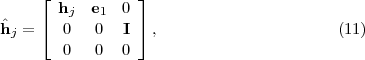
 j
yield the vector δtjϕj(-iδthj)e1. The exponentiation is
computed using a public domain Padé routine for general matrices,
combined with scaling and squaring [33].
j
yield the vector δtjϕj(-iδthj)e1. The exponentiation is
computed using a public domain Padé routine for general matrices,
combined with scaling and squaring [33].
The procedure outlined above is repeated for each of the ϕj(-iδtHI)Uj terms in the summation on the right-hand-side of eq.(8). Summing these nj terms and adding to the first term on the right-hand-side of eq.(8) provides a means of propagating the wave function in region I forward one step in time.
Test phase for tasks C and D:
The accuracy of the adapted Arnoldi method for calculating the action of the ϕj(-iδtHI) functions on the Uj(t) vectors was verified by mocking up Uj(t) vectors and comparing results to those calculated using direct methods which include explicit inversion of HI. Excellent agreement was found between the two independent methods.
By this stage the single core version of the RMT program was fully constructed. The many-electron wave function is known at time t + δt throughout regions I and II and further propagation in time can progress by repeating, for successive time steps δt, the procedures described in the previous sections.
| ||||||||||||||||||||||||||||||||||||||||||||||||||||||||
Once the single core version of the RMT program was fully constructed, its accuracy was verified by using it to investigate electron wavepackets ejected from Ne (which has 10 electrons) irradiated by an XUV laser pulse. All calculations at this stage were performed on local machines at QUB. Results were compared to those calculated using the TD-RA program in which there is no division of position space occurring. The parameters used for these first RMT test calculations can be found in the ‘Ne set A’ list in the appendix of the report. The TD-RA calculations used the same parameters except that, because there is no region II included, the boundary of region I was increased to 100 a.u. and the number of B-splines per angular momentum, l, increased to 100. The partial continuum wave functions of Ne calculated after the end of the laser pulse using the RMT method were compared to those calculated using the TD-RA method. The same test calculations were carried out using ’Ne set B’ as input so that the continuum wave functions coupled to an excited residual ion state could be compared. This comparison of time-dependent wave functions obtained using the mixed basis/finite-difference RMT method with those obtained using a pure basis set method represents one of the most stringent tests of accuracy for the new RMT method. The excellent agreement between the results of the two independent methods helps verify the accuracy and reliability of the RMT program.
|
|
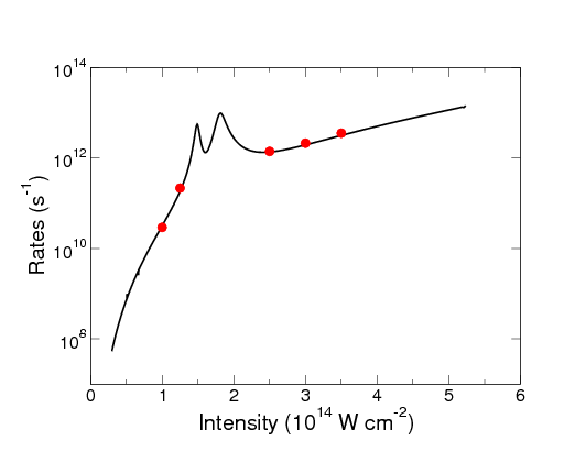
As a second means of demonstrating the accuracy of the RMT method, single-electron ionization rates were calculated for He and Ne irradiated by a laser pulse with a central wavelength of 248 nm (corresponding to the fundamental wavelength of the KrF laser). These rates were compared with rates obtained using the time-independent R-matrix Floquet (RMF) method and, in the case of He, also with those obtained using the HELIUM code. For the He calculations the parameter set ’He’ was used and for the Ne calculations ’Ne set A’ was again used. These parameter sets can be found in the appendix. Table 1 shows a comparison of He single-electron ionization rates for three intensities. Away from resonances, the ionization rates calculated by RMT agree well (to within 10%) with those calculated by HELIUM [35] and by the RMF method [36]. Figure 3 shows the comparison of Ne single-electron ionization rates. Agreement between the two sets of results is very good, typically within 10% of each other away from resonance.
This section describes the implementation of a parallel RMT program employing MPI together with tuned BLAS and LAPACK library routines. In the parallel RMT program processes are assigned to two functional groups: 1) the TD-RA group of processes calculates the wave function in region I at each time-step, and 2) the TD-OUTER group of processes calculates the wave function in region II at each time-step. Two-way exchange of data between the two groups occurs via synchronous point-to-point communication between the master cores in each of the groups. The approach scales well provided computational load is adequately balanced across the two groups. Results are stored to disk periodically for analysis and to provide a restart procedure.
The TD-OUTER group is parallelized by assigning a number of grid points to each core in the group, so that the first core handles the first XLast grid points, the second core the next XLast grid points and so on. Each compute core in the TD-OUTER group is thus responsible for a wavefunction array of dimension np × XLast where np is the number of channels retained in the calculation.
Because the derivative operators in Hti have been replaced with 5-point FD operators, communication between cores in calculating HtiF is limited to nearest neighbour communication only.
Parallelization within the TD-RA group has focused on the two most CPU-intensive routines of the serial RMT code. These are the Arn-Matrix-Vector-Multiply subroutine of the inhomogeneous Arnoldi algorithm and the WV-Matrix-Vector-Multiply subroutine called during the evaluation of the wave function on the FD points within region I.
Parallel-Arn-Matrix-Vector-Multiply
Unlike the FD Hamiltonian in region II, the elements of the block-tridiagonal Hamiltonian matrix, HI, in region I are not calculated on the fly which means that options for parallelizing the matrix-vector kernel of the inhomogeneous Arnoldi algorithm are more restrictive. Instead all matrix elements are read from files written to disk by RMATRX2. At start-up, the master core in the TD-RA functional group is the only core that reads the files written by RMATRX2. Once all the HI matrix elements have been read, the strategy used here is to map the block rows, along with the corresponding segment of the Uj vectors being multiplied into, onto a group of cores that are from here on referred to as Block Master Cores (BMCs). This already places constraints on the minimum number of cores needed to run the program as at least one core should be available for each LSπ symmetry block. Once distributed, two dense dipole matrix blocks of size mnp1symi × mnp1symj and a 1D array of eigenvalues of length mnp1symi sit on each of the BMCs. At this coarse level of distribution, the Parallel-Arn-Parallel-Matrix-Vector subroutine can already be implemented using BLAS library routines. Load-balancing within the TD-RA group is accomplished by ensuring that each block row is assigned the same number of cores and by forcing mnp1symi = mnp1symj by padding the symmetry blocks with zeros (for most input data sets mnp1symi ≈ mnp1symj). Increasing the number of cores within the TD-RA group results in multiple cores being assigned to each block row of HI. Due to the off-diagonal block structure of HI two-way exchange of arrays of length mnp1symi occurs between each BMC during each call to Parallel-Arn-Matrix-Vector-Multiply.
Parallel-WV-Matrix-Vector-Multiply
At start-up the eigenvectors, V k, associated with each eigenstate, k, of HI are distributed to the BMCs. As soon as the compute cores in the TD-RA group evaluate their updated segment of Ck(t + δt), an MPI GATHERV is called so that the Ck(t + δt) are collected onto the BMCs. The BMCs subsequently call the Parallel-WV-Matrix-Vector-Multiply subroutine to calculate the Fp value required at each FD point within region I. The wave function values are then gathered onto the master core in the TD-RA group to be sent to the master core in the TD-OUTER group.
During propagation, communication between TD-RA and TD-OUTER occurs between the master core in TD-RA (MCR1) and the master core in TD-OUTER (MCR2). The communication is based on synchronous MPI SEND/RECV calls. The communication calls occur in the following sequence:
At the start of each time-step, MCR1 sends to MCR2 an array, Fin, containing the radial wave function at time t at FD points within the R-matrix boundary. Upon MCR2 receiving this array, propagation over one time-step in TD-OUTER can proceed. Therefore, within a single time-step one SEND/RECV call is made between MCR1 and MCR2 for communication from TD-RA to TD-OUTER.
Within a single time-step, MCR2 calculates a Uj vector for each order j, where 0 < j ≤ jmax. Once MCR2 has finished calculating a given Uj vector, it sends the vector to MCR1. Therefore, the number of SEND/RECV calls made between MCR2 and MCR1 within a single time-step for communication from TD-OUTER to TD-RA is jmax (typically jmax = 12-14). Upon MCR1 receiving a Uj vector, it can proceed with calculating the corresponding ϕj vector. Once all of the ϕj vectors have been calculated, the C coefficients at t + δt can be calculated.
The above sequence of calls is repeated for each time-step of the propagation.
Load-balance between TD-RA and TD-OUTER
For efficient scaling of the RMT code, computational load needs to be well balanced across the two functional groups TD-RA and TD-OUTER.
To minimize idle time in TD-RA, MCR2 needs to send the Uj vectors to MCR1 in synchronization with the calculation of the ϕj vectors – As soon as ϕj-1 is calculated, MCR1 is waiting to receive Uj from MCR2 in order to proceed with the calculation of ϕj.
For a given problem size, there are only two adjustable parameters in the RMT code that can influence load balance between the TD-RA and TD-OUTER groups. The first is the number of cores assigned to the TDRA group, nctdra. The second is the number of FD points allocated to each core in TD-OUTER, XLast. If the values of nctdra and XLast are chosen too large the amount of time spent idle on each core within the TD-RA functional group will increase. If nctdra or XLast are chosen too small the amount of idle time within the TD-OUTER functional group will increase. The optimal values for nctdra and XLast can be found by using timing routines in TD-RA and TD-OUTER along with using the CRAYPAT profiling tool.
The RMT code was ported to HECToR in January 2011. An RMATRX2 suite of codes was also ported to HECToR at the same time so that relevant ‘starter’ data could be generated. The results shown here were produced by compiling the RMT code with the PGI Fortan 90 compiler. The CRAYPAT profiler was used to analyze the initial performance of the RMT code on HECToR.
Comparison with single core version of RMT:
The first runs of the parallel RMT code used the ’Ne set A’ and ’Ne set B’ parameter lists as input. Results were shown to be in excellent agreement with the results produced employing the serial version of the RMT code, run both on the QUB machines and a single core of the XT6. The output of the parallel RMT code was found to agree with the output of the serial version of the code to the level of machine precision.
Scalability:
To test the scalability of the RMT code, several test runs were performed on various numbers of cores on the HECToR XT6. The maximum number of cores allocated to the functional group, TD-OUTER, during this initial test phase was 384. The maximum number of cores allocated to the functional group, TD-RA, was 48, giving 432 as the maximum total number of cores allocated to a run of the RMT code. All of the scaling tests were carried out using the ’Ne set C’ parameter list in the appendix which to date represents the largest problem size used as input to the RMT program. With this set of parameters, there are 17 residual ion states (resulting in 687 coupled channels) included in the calculation with a HI dimension of ~35000 × 35000.
Table 2 shows how the RMT code scales with increasing number of cores allocated to the TD-OUTER functional group. The value of XLast is held fixed, so that an increase in the number of cores results in a linear increase in the volume of integration in region II. The time per iteration is shown for two values of XLast, where increasing XLast by a factor of ~ 4 from 150 to 600 results in a corresponding factor of 4 increase in the time taken per iteration. For both sets of calculations, 24 cores were allocated to the TD-RA functional group. It can be clearly seen that weak scaling with up to 384 cores in the TD-OUTER group is good on the XT6.
|
| |||||||||||||||||||||||||||||||||||||||||||||||||||
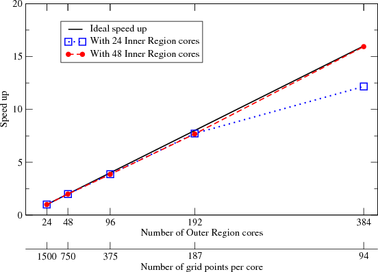
Figure 4 shows how the RMT code scales with increasing number of cores allocated to the TD-OUTER functional group for a fixed total number of grid points. The calculations were carried out using ’Ne set C’ as an input parameter set, where R is fixed at 7200 a.u. – with a FD grid spacing of 0.2 a.u., this fixes the total number of grid points to 36000. Figure 4 demonstrates that as the number of cores allocated to the TD-OUTER group is doubled, the number of grid points per core, (XLast) is halved. The first scaling analysis was carried out with 24 cores assigned to the TD-RA group. In this case, with 384 cores assigned to the TD-OUTER group speed-up is seen to diverge from ideal. This is because the time spent idle on the cores in the TD-OUTER group has increased, whilst there is little idle time within the TD-RA group. Once 48 cores are assigned to the TD-RA group, the amount of idle time in the TD-OUTER group decreases and speed-up is seen to return to ideal.
Load-balancing:
By carrying out a load-balancing analysis using timing routines and CRAYPAT, an optimum value of XLast can be found for a given number of cores allocated to the TD-RA functional group. Using ’Ne set B’ input data, the optimal value of XLast for 24 (48) cores allocated to TD-RA was found to be 144 (89).
|
|
In order to demonstrate the capability of the RMT code, calculations were carried out to study the interaction of Ne with an XUV attosecond light pulse in the presence of a 800 nm Ti:Sapphire laser field. Such an interaction has recently been studied experimentally where complex many-electron effects within Ne are suspected to be the reason for an unexpected time delay between the escape of a 2p electron and a 2s electron. Using “attosecond streaking” methods, the experiment has measured this time delay to be 21 attoseconds. So far, no theoretical method has been able to provide a value for the time-delay that even comes close to matching the experimental value. Initial calculations of the time delay demonstrate that such precise phase-sensitive information can be calculated with the new RMT program.
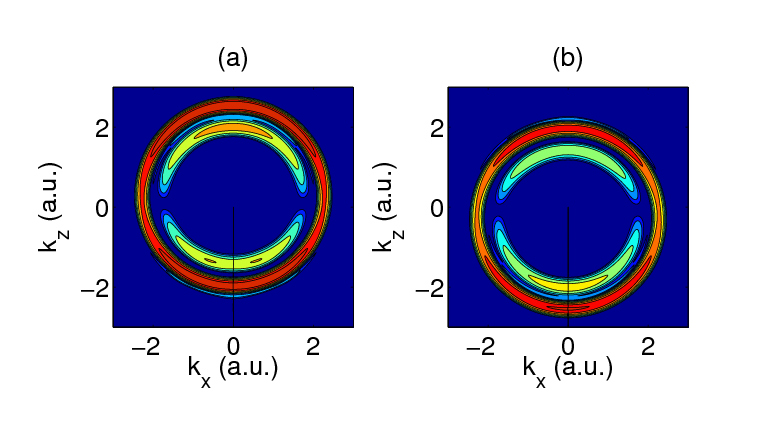
In the RMT calculation the 800nm field is a 3 cycle pulse of peak intensity 1013 W/cm2. The 91 eV XUV pulse is a 14 cycle pulse also of peak intensity 1013 W/cm2. Figure 5 shows the 2D momentum distributions of ejected electron wave-packets from Ne for two different delays between the XUV and the IR fields. The XUV field is at its peak in figure 5(a) at 1.25 cycles into the IR field, and in figure5(b) at 1.75 cycles into the IR field. In (a) the IR field imparts, to the ionizing electron wavepacket, positive momentum in the z-direction, while in (b) it imparts a negative momentum in the z-direction. Consequently the kxkz momentum distribution is shifted upwards in (a) and downwards in (b) as compared to the distribution symmetric about the kz=0 axis obtained when there is no IR field present.
Both (a) and (b) figures show contributions to the momentum distribution from electrons liberated from the 2p subshell (outer circle) and from the 2s subshell (inner circle). It is worth noting that the due to the RMT code’s ability to explicitly include multiple residual ion states in the calculation, it is one of the few methods worldwide that is capable of describing the momentum distributions of the ejected 2p and 2s electrons in a single calculation. By performing further calculations with various delays between the fields it is observed that the inner and outer circles oscillate between their positions in (a) and (b). Analysis of these oscillations reveals an ultrashort time delay in photoemission from the two valence states (2p and 2s). It is the intention of the authors to present full details of these exciting results at the XXVII International Conference on Photonic Electronic and Atomic Collisions (ICPEAC) 2011 conference and subsequently to submit results for publication in a peer reviewed journal.
This report has described the construction of a powerful new ab initio RMT code that has the unique capability to accurately and efficiently describe the single ionization response of a general many-electron atom exposed to intense laser light pulses. The construction of the RMT code has been made possible by implementing the numerical methods and algorithms underlying two well-established ab initio codes, namely HELIUM and the RMATRX2 suite of codes. The RMT code has immense flexibility since it can not only describe the response of a general many-electron atom to intense laser light fields with wavelengths ranging throughout the spectrum, from the extreme ultraviolet to the infrared, but also to both short- and long-duration pulses of such light.
The construction of the RMT code constitutes a major algorithmic advance that represents a vital first step in the development of a method that is capable of accurately describing the single ionization response of a many-electron molecule to intense laser light and later, the double-electron ionization response of a many-electron atom exposed to such light.
The accuracy of the new code has been verified by using it to calculate single ionization rates for He and Ne irradiated by a KrF laser pulse. In the limit of many-cycle laser pulses, a regime in which R-matrix Floquet (RMF) theory is valid, results from the RMT code and RMF code have shown excellent agreement. In the case of He, RMT code results were also shown to be in excellent agreement with those produced by the HELIUM code.
A description of the parallelization of the RMT code and its porting to the HECToR Cray XT6 has been provided. Running the parallel RMT code on the XT6 machine has already revealed the code’s potential to accurately describe the effects of highly complex correlated electron dynamics on the ultrafast photoemission of electrons from many-electron atoms when exposed to a combination of XUV and 800 nm laser light.
The report also provides a performance and load-balancing analysis of the new code on the XT6. The RMT code has been shown to scale well, provided computational load is balanced between the TD-RA and TD-OUTER functional groups working on region I and region II of the electronic position space.
However, modifications to the code need to be made in order to maximize performance on the current generation of high-end computing machines such as the HECToR Cray XT6, typically containing many thousands of multi-core processors. Improvements to parallel scaling performance, single node efficiency and memory usage will enable very large laser-atom and laser-ion calculations to be addressed on these machines. Such large-scale calculations are essential to complement the sophisticated laboratory-based experiments being carried out around the world in the field of Attosecond Science. In particular, effective load balancing between the TD-RA and TD-OUTER functional groups will be paramount to the future use of the RMT method in the investigations of the double ionization of atoms to intense laser fields. The optimization of the RMT code for use on HECToR will be the focus of an upcoming 6-month dCSE project.
The authors would like to thank the following people for their contributions to this work:
Prof. K. T. Taylor, Queen’s University Belfast
Dr. J. S. Parker, Queen’s University Belfast
Dr. H. W. van der Hart, Queen’s University Belfast
Dr. L. A. A. Nikolopoulos, Dublin City University
Dr. M. Plummer, STFC Daresbury Laboratory
This project was funded for 24 months under the HECToR distributed CSE (dCSE) programme, which is provided through The Numerical Algorithms Group (NAG) Ltd. LRM was funded for the first 6 months of the project to work on the FD-OUTER program. MAL was funded for the remaining 18 months of the project.
|
| ||||||||||||||||||||||||||||||||||||||||||||||||||||||||||||||||||||||||||||||||||||||||||||||||||||||||||||||||||||||||||||||||||||||||||||||||||||
[1] P. Corkum and F. Krausz Nat. Phys. 3, 381 (2007)
[2] F. Krausz and M. Ivanov Rev. Mod. Phys. 81, 163 (2009)
[3] S. Baker et al Science 312, 424 (2006)
[4] L. E. Chipperfield et al Phys. Rev. Lett. 102, 063003 (2009)
[5] M. Uiberacker et al Nature 446, 627 (2007)
[6] E. Goulielmakis et al Nature 466, 739 (2010)
[7] M. Schultze et al Science 328, 1658 (2010)
[8] N. Dudovich et al Nature Physics 2, 781 (2006)
[9] H. J. Wörner et al Nature 446, 604 (2010)
[10] K. P. Singh et al Phys. Rev. Lett. 104, 023001 (2010)
[11] H. Wang et al Phys. Rev. Lett. 105, 143002 (2010)
[12] Y. Zeng et al Phys. Rev. Lett.103, 043904 (2010)
[13] Y. Nabekawa et al Phys. Rev. Lett.102, 213904 (2009)
[14] E. Takahashi et al Phys. Rev. Lett.104, 233901 (2010)
[15] J. Vura-Weis et al Science 328, 1547 (2010)
[16] M. Stockman et al Nature Photonics 1, 539 (2007)
[17] H. B. Gray and J. Halpern Proc. Nat. Ac. Sci. 102, 3533 (2005)
[18] P. Corkum Phys. Rev. Lett. 71, 1994 (1993)
[19] T. Brabec and F. Krausz Rev. Mod. Phys 72, 545 (2000)
[20] M. Lewenstein et al Phys. Rev. A 49, 2117 (1994)
[21] G. Sansone et al Science 314, 443 (2006)
[22] W.E. Arnoldi Quart. Appl. Math. 9, 17 (1951)
[23] T.J. Park, J.C. Light J. Chem. Phys. 85, 5870 (1986)
[24] E.S. Smyth, J.S. Parker, K.T. Taylor Comput. Phys. Commun. 114, 1 (1998)
[25] J.S. Parker et al Phys. Rev. Lett. 96, 133001 (2006)
[26] L.A.A. Nikolopoulos, J.S. Parker, K.T. Taylor Phys. Rev. A 78, 063420 (2008)
[27] P.G. Burke, K.A. Berrington Atomic and Molecular Processes: An R-matrix Approach, (IOP Publishing, Bristol) (1993)
[28] P.G. Burke, V.M. Burke, K.Dunseath J. Phys. B: At. Mol. Opt. Phys. 27, 5341 (1994)
[29] A. G. Sunderland et al Comp. Phys. Commun. 145, 311 (2002)
[30] A. G. Sunderland, C. J. Noble and M. Plummer dCSE Technical Report (2010)
[31] B. Skaflestad, W.M. Wright Appl. Numer. Math. 59, 783 (2009)
[32] M. Ndong, H. Tal-Ezer, R. Kosloff. C.P. Koch J. Chem. Phys. 130, 124108 (2009)
[33] R. Sidje ACM Trans. on Math. Soft. 24, 130 (1998)
[34] Y. Saad SIAM J. Numer. Anal. 29, 209 (1992)
[35] J.S. Parker et al J. Phys. B: At. Mol. Opt. Phys. 33, L239 (2000)
[36] D.H. Glass, P.G. Burke J. Phys. B: At. Mol. Opt. Phys. 32, 407 (1999)
[37] P.G. Burke and K. T. Taylor J. Phys. B: At. Mol. Opt. Phys. 8, 2620 (1975)
![∑ [ ]
i ∂-Fp(r,t) = Hti (r)Fp(r,t) + WE ′(r)+ WD ′(t) + WP ′(r,t) Fp′(r,t) (3)
∂t p p′ pp pp pp](nag_report_for_web4x.png)