Abstract:

The laser-driven helium atom is a nearly ideal system for both experimental and theoretical exploration of quantum mechanical correlation and quantum mechanical energy exchange between matter and light. Non-classical correlation (also called entanglement) is one of the most mysterious and anti-intuitive features of the quantum mechanical universe. For example correlation, in the form of entangled qubits, is at the heart of most formulations of quantum computing, and correlated photons are what makes quantum cryptography feasible. Correlation is something shared between particles. In the case of laser-driven helium we are concerned with correlation between pairs of electrons ejected from the atom by the strong laser fields, a process called non-sequential double-electron ionization (NSDI). NSDI is a subtle effect, deeply buried within the integrated atomic wavefunction, but it reveals in detail important features of the ionization dynamics of correlated quantum mechanical systems [1, 2, 3].

Helium - the simplest of all multi-electron atoms - is the only multi-electron atom for which rigorous (quantitatively correct) numerical solutions of the full-dimensional equations of motion (Schrödinger’s equation) can be obtained. Laser-driven hydrogen is similarly susceptible to rigorous study numerically, but hydrogen’s single electron cannot exhibit the correlation effects that make multi-electrons of such interest. The physics of single electron atoms driven by high intensity laser radiation has been well understood for many decades. Helium turned out to be very different in this respect - every high integrity solution of the helium Schrödinger’s equation we obtained revealed effects that were unpredicted, surprising and unexplained.

HELIUM [4] is a code that solves the non-relativistic time-dependent Schrödinger equation for a two-electron atom or ion exposed to intense linearly-polarised laser fields - a time-dependent 5-dimensional partial differential equation. The HELIUM time propagator was designed to meet a requirement for unusually small integration truncation errors. This requirement stems from, among other things, difficulties encountered modelling non-sequential double-electron ionization (NSDI). A typical integration might for example find total NSDI yields of the order 10^-8 or even 10^-12, constraining local truncation errors to considerably less than 10^-12 in a wavefunction normalised to unity. This requirement may be impossible to meet with low order integration schemes. For this reason HELIUM uses an arbitrary-order Arnoldi propagator [4]. The Arnoldi propagators often demonstrate improved integration efficiency in the limit of high order even if small truncation errors are not a requirement.

In this report we discuss software developments aimed at improving our ability to model and analyse the exchange of energy between the laser and atom during the production of these correlated pairs in NSDI. These developments include a generalised HELIUM, and new methods to analyse the wavefunctions generated by HELIUM. Discussion of details begins in section 1 below.

Contents

1 Objectives and Outcomes

In section 2 (J.Parker) we discuss the implementation of a new code that extends the present HELIUM to use generalized laser polarization. The implementation was successful and we discuss the new self-test modules for the generalized matrix elements used by the new code. The design allows the new code to turn off the new feature so that it behaves identically to HELIUM if linear polarized fields are used. Testing of the new code against the current version of HELIUM verified that behaviour is identical for a single linearly polarized laser field polarised along either the z-axis or the x-axis.

One of the surprising (and welcome) outcomes of this project, was the observation that on HECToR, the performance exhibited better-than-linear scaling as we changed processor (core) count from 253 to 8001. In other words, the program might be predicted to run a factor of 8001/253 faster on 8001 cores than on 253 cores. Instead it ran almost a factor of four faster than this prediction. We attribute this to the fact that on 253 cores the local arrays (on which the computation is performed) were too large to fit in the L2 cache, and hence spilled out into slower memory. By contrast, on 8001 cores, the local arrays were small enough to be contained within the L1 cache, the CPU’s fastest memory.

In section 3 (E.Smyth) we discuss implementation of hybrid MPI-OpenMP parallelism in HELIUM, which may become essential to allow all cores on a node to be utilised as memory per core falls at the same time as the changes in section 2 will require larger angular momentum basis sets.

In section 4 (J.Parker) we discuss implementation of a new post-processing code to transform output from HELIUM (in spherical geometry) to cylindrical geometry. The new software runs on the same number of processors (cores) as HELIUM runs on, which on HECToR is typically an arbitrary number up to about 16,000 cores. The program performs correctly, and has been successfully tested on a single coupled spherical harmonic, pairs of coupled spherical harmonics with known analytic expressions in cylindrical coordinates, and on the HELIUM ground state, (which is composed of a set of 6 coupled spherical harmonics). Two of these tests are discussed in section 4.

In section 5 (J.Parker) we discuss the implementation of a multistage algorithm for the transformation of the final-state wavefunction from configuration space to momentum space. A number of tests are discussed, along with performance measurements on HECToR. Three new methods, each with its own advantages, have been developed. Tests on HECToR have verified that all four methods, the 3 new methods and the old method, give identical results on a range of core counts. Operation of the new methods on a very large full size wavefunction (8001 processors) is discussed in more detail in section 5, and benchmark timings are presented. The latest incarnations of HECToR have been able to run the old method successfully on this core count. Nevertheless, the newer methods are substantially faster.

The accuracy of the momentum space transformation code has been enhanced by incorporating Coulomb functions into the current Bessel function basis set. We have written a new program for numerically integrating Coulomb functions, based on an arbitrary order Taylor series propagator. The new software performs correctly. Tests include orthonormality checks, comparison with the asymptotically correct formulae, and comparison with the results of independently written code (a public domain integrator based on low order Numerov method).

As a substantial test of the new software, and as a demonstration of the importance of a rigorous quantitative analysis of final-state energy distributions, we have applied the new software suite to a problem that has proved challenging both to theorists and to experimentalists. The results are discussed in section 4. A surprising outcome of this exercise is the finding that the new software allows us to solve the difficult problem in three largely independent ways, and with nearly identical results. The old method failed at this problem.

As outlined in the abstract, the scientific research enabled by HELIUM’s ability to exploit HECToR is important and unique. The developments described above greatly expand HELIUM’s versatility; some of the new science already enabled by the new software is described in section 5. HELIUM has always been a heavy user of HECToR, and as a result the improvements in runtime performance reported in sections 2 and 5 will have a beneficial impact on the HECToR user community, by improving HELIUM’s ability to efficiently use HECToR resources.

2 Work package 1. Extensions to HELIUM to allow calculations with crossed laser fields

In the original program HELIUM the laser light is assumed to be linearly polarised, which effectively removes a degree of freedom from the dynamics - the problem becomes a 5-dimensional time-dependent partial differential equation. In this section we describe the implementation of an extended version of HELIUM that allows a second laser perpendicular in polarisation to the first. This removes the rotational symmetry exploited in the original HELIUM program. The problem reverts to the fully general 6-dimensional time-dependent Schrödinger equation for laser-driven helium.

In HELIUM [4] the angular dependence of the two-electron wavefunction is handled through a basis set expansion of coupled spherical harmonics in which l_1,2 are angular momentum values of each electron, L is the total (orbital) angular momentum and M its z-component. The wavefunction takes the form:

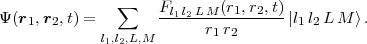(1)

where the F_{l1 l2 LM}(r₁,r₂,t) are time-dependent radial functions to be determined in the calculation. Through the orthonormality of the , one obtains from the time-dependent Schrödinger equation with Hamiltonian H a set of time-dependent coupled two-dimensional radial equations for the functions F_{l1^′l2^′L^′M^′}(r₁,r₂,t), viz:

Originally we planned to use the velocity gauge in implementing the interaction Hamiltonian, but recent experience with the length gauge interaction Hamiltonian convinced us that the length gauge is more efficient, less error prone and just as accurate. Improved efficiency is of crucial importance in the crossed fields problems because of the increased difficulty integrating over the higher dimensional space. For a particular laser intensity, we might see an order of magnitude or more increase in the size of the basis set of partial waves for convergence (compared to HELIUM, which uses linearly polarised light). For that reason the implementation uses the length gauge.

Taking the polarisation axis of the first laser as the z axis, and the polarisation axis of the second laser as the x axis, we have for their respective electric fields:

(3)

where f(t) and g(t) are time-dependent envelope functions; ω_1,2 are laser frequencies and δ_ω1,2 corresponding phase shifts.

The second laser field brings in the additional Hamiltonian terms:

(4)

where the summation runs over both electrons and e is the electric charge of the electron. These new Hamiltonian terms will in turn introduce matrix elements of the form

By allowing a completely arbitrary choice of the four angular quantum numbers |l₁l₂LM >, the new program can generate solutions to fully general 6-dimensional Schrödinger equation for (non-relativistic) 2-electron atoms. The original HELIUM program is restricted to linearly polarised light, which allows us to fix the M quantum number to a constant. In practice, the M quantum number is set to 0 in HELIUM.

Testing HELIUM_X_FIELDS:

The new crossed fields code, called HELIUM_X_FIELDS has been completed and tested on single processor workstations, the eight cores of a multiprocessor workstation, on 48 cores of a workstation cluster, and on 253 to 8001 cores on HECToR. As part of the testing program, we verify that the numerical integration produces the same results independently of core count.

The x-direction (crossed field) laser can be toggled on or off with the following parameters:

module Laser_Interactions
Logical, parameter :: USE_Crossed_Field_Interaction = .True.
Logical, parameter :: USE_z_Polarised_E_Field = .True.
end module Laser_Interactions

If the first parameter above is set to .False., then the program reverts to the original HELIUM program. This provides a convenient test: we can verify that the numerical integrations performed by HELIUM and HELIUM_X_FIELDS are identical. If the first parameter above is set to .True. and the second to .False. we again produce a program with a linear polarised laser like HELIUM, but with polarisation in the x direction only. Again we verify that HELIUM and HELIUM_X_FIELDS produce identical physical results, (allowing for the 90 degree rotation; the HELIUM program uses z-polarised fields.)

The major modules in HELIUM and HELIUM_X_FIELDS (including the Communications MPI modules and the finite-difference modules) contain self-test routines, some of which are executed at start-up every time HELIUM is run. The most elaborate of the start-up tests verify that the elements of the basis set of partial waves satisfy the desired constraints, that the physical selection rules (allowed transitions between states) are correct, that the Hamiltonian parameter arrays are correctly initialised, and that the matrix-elements have been correctly calculated. The matrix-elements of the angular part of of the problem, < l₁′l₂′L′M′|r_j sinθ_j cosϕ_j|l₁l₂LM >, can be formulated in terms of products of 3-j and 6-j symbols [5]. The test routines calculate the 3-j and 6-j symbols several different methods using equations 2.12, 2.18, 2.22, 2.24, 2.24 and 2.25 of [5]. Comparison of the results can detect programming errors, or degraded accuracy in difficult limits (large l_j for example). The most exhaustive is a set of matrix-element tests that runs for about an hour on a typical processor, and is disabled during normal runs of HELIUM_X_FIELDS. This test routine calculates (among other things) the matrix-elements < l₁′l₂′L′M′|r_j sinθ_j cosϕ_j|l₁l₂LM >, by two independent methods. The first method uses a summation of products of three 3-j symbols using equ. 2.20 of Ref. [5]. The second method uses the HELIUM_X_FIELDS standard approach: a product of a 6-j and 3-j symbols.

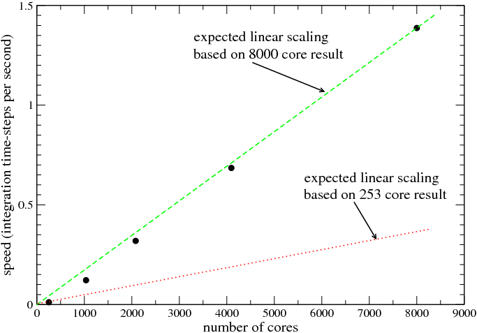
During testing on HECToR we collected data on the performance of HELIUM_X_FIELDS as a function of core count. Figure 1 shows the number of time-steps HELIUM_X_FIELDS can perform per second. The program is compiled with Portland Group pgf90 compiler using the -fastsse -O3 optimisation switches. Performance is measured on 253, 1035, 2080, 4095 and 8001 cores. In each case the same problem is solved - the integration is performed in the same size integration volume (with minor variations), so that the total number of floating point operations done by HELIUM_X_FIELDS (in each of cases plotted in Fig. 1) is to good approximation independent of core count. On 1035 cores, each core operates on a 128x128 subset of the global grid. On 4095 cores each core operates on a 64x64 grid. It is clear that on 8001 cores the problem can be integrated in somewhat less than half the time required on 4000, i.e. the scaling is better than linear.

Better than linear scaling (or super-linear scaling) is one of the potential benefits of parallel processing. If message passing overhead were negligible, then we would expect to see this kind of scaling rather more often, because the on-core data arrays decrease in size as the problem is spread across more cores, so that (for sufficiently large core count) the data arrays fit inside the CPU’s fastest RAM cache. If by contrast the data arrays on which the computation is performed reside in the slowest RAM, then floating-point operations per second may drop dramatically as more time is spent fetching data from memory. On 8001 cores the on-core (complex number) grids are 46x46, or small enough to fit in the CPU’s 64K byte L1 cache. On 253 cores the on-core grids are 262x262, or too large to fit in the CPU’s 512K byte L2 cache. HELIUM_X_FIELDS is sensitive to the speed of memory access, so super-linear scaling was the result we were hoping for.

We can see this more clearly by working through the numbers in Fig. 1. On 253 cores, the time per integration step is 1 / 0.011338 = 88.2 sec. If the scaling were linear, then we would expect the time per step on 8001 cores to be 88.2 * (253 / 8001) or 2.79 sec. In fact the measured time per step on 8001 cores is 0.72 sec. In other words the 8001 core integration runs almost a factor of 4 times faster than the prediction obtained by scaling the 253 core result linearly. Speed-up this dramatic is rarely seen because it requires an unusually high message passing bandwidth, and simultaneously an unusually large number of cores to make the on-core grids sufficiently small.

3 Work package 2. Implementation of a hybrid MPI-OpenMP parallelism in HELIUM

The very first version of the HELIUM code, run on the Cray T3D and T3E systems in the 1990s, was parallelised over the basis set of coupled spherical harmonics. A later version modified the parallelism to be over the 2-D radial grid. The advantage of parallelising over the radial grid is that all communication is then either nearest-neighbour halo exchange or global summation operations, rather than the much more complicated interactions between different basis states. This also improved the load balancing, as the work load varies considerably for different basis states while the workload for different radial blocks is almost constant. The radial parallel HELIUM code has been used very successfully for many years on both HPCx and HECToR, and has been shown to scale very well to over 70k cores.

The purpose of this workpackage was to look at re-enabling parallelism over the basis set as a complement to the current MPI parallelism over the 2-D radial grid. The motivation for enabling this extra level of parallelism within HELIUM is as follows:

1: 

To allow the option to scale to higher core counts for a given problem size, so as to reduce the time to solution.

2: 

To investigate if a hybrid parallelism approach could be a more efficient means of utilising the same number of cores.

3: 

Most importantly, we have seen a reduction in the amount of memory on HECToR on a per core basis from 3GB/core on the Phase 1 system to 1.33GB/core on the current Phase 2b system and to just 1GB/core on the planned Phase 3 system. Meanwhile, other changes to the code (workpackage 1) will significantly increase the size of the basis set used, requiring more memory per core. The memory needed per core can be reduced by reducing the size of the radial block per core, but there are practical limits to doing so, and a radial block size of about 9x9 is the minimum possible. Without parallelising over the angular basis states as well, there is a risk that runs on HECToR (or any similar system) will in future have to leave cores idle due to insufficent memory, thus wasting compute resources.

Shared memory parallelism techniques (specifically OpenMP) were chosen to parallelise over the basis states instead of a distributed memory approach such as MPI, to avoid additional data storage requirements for communication buffers and to minimise the code modifications needed. Due to delays starting this workpackage, the target system changed from the quad-core upgrade to the XT4 to the current XE6 system with 24-core nodes and Gemini interconnect. The 24-core nodes comprise two separate 12-core chips. However, from a programmers perspective it is better to consider it as four 6-core ”dies”, all sharing memory but with NUMA performance considerations if the OpenMP threading is extended over more than one die [6]. Thus, to avoid the complications of NUMA we will limit the OpenMP threading to a maximum of 6 threads and use the appropriate options to aprun to place MPI tasks so that all threads associated with a specific MPI tasks reside on the same die.

Code changes

The bulk of the work was applied to the Arnoldi propagator as this is used for most production runs. Addition parallelism was added to the calculation of global acceleration and correlation as this was easy to add, though not essential for performance. The modifications were as follows:

1: 

All communication between MPI tasks (halo exchange and global sums) are performed by the master OpenMP thread. This is the simplest and most reliable scheme to implement MPI communication within a threaded code.

2: 

Within the Arnoldi propagator there is a single parallel region covering all of the computation. Calls to the subroutine Ham_x_Vector were replaced by a SMP specific version to allow the local arrays in Ham_x_Vector to be replaced by arrays declared at the top level of the Arnoldi propagator. This is essential to allow these arrays to be shared between the OpenMP threads. Functions used to calculate global sums were replaced by similar subroutines to make it more straightforward to understand the OpenMP shared status of the result.

3: 

Parallelism over all the states in the basis set is straightforward to implement via OpenMP DO directives. The workload varies considerably per thread, however the relatively small scale parallelism (e.g. 6 threads processing thousands of basis states) means that load balancing should not be a significant problem even with the standard static scheduling of loop iterations. More advanced scheduling options are easy to implement if required - a key advantage of shared memory parallelism.

4: 

The calculation of eigenvalues and eigenvectors in the small Krylov subspace is duplicated to avoid the need to share the result from this relatively tiny calculation across all threads i.e. to make the result local to the caches on each core for subsequent use updating that thread’s portion of the global wavefunction.

Other propagators and the diffusion equation version of the Arnoldi propagator used for the initialisation could also be parallelised in this way if desired.

Allowing larger basis sets

The number of basis sets that can run on HECToR will depend upon not only the radial block size chosen but also the choice of propagator used and the options set for that. All tests here used a 6th order Arnoldi propagator and the number of radial blocks was set to 20, giving a total of (20x21)/2 = 210 MPI tasks. The maximum number of states successfully used for different radial block sizes were:

The scaling in the number of states possible is not linear with the increase in memory available by running fewer MPI tasks per node. Further investigation would be required to understand in more detail where memory is required within the code (including e.g. buffers needed within the MPI libraries) to see if memory utilisation could be reduced further, to allow even larger basis sets to be used. Nevertheless, using a hybrid MPI-OpenMP version allows considerably larger basis sets to be used without leaving cores idle compared to a pure MPI version.

Efficiency on the same number of cores

The second issue to test is whether or not a hybrid version could be more efficient running on the same number of cores to solve the same problem. The options available within HELIUM make it difficult to use exactly the same number of cores. To simplify this task, we use just 16 cores per node, making sure that we use 4 per die either as 4 MPI tasks or 4 OpenMP threads. Even though the number of cores is not identical, all these jobs will take up 35 nodes on HECToR, so the cost per hour of running these jobs will be the same. Run times below (in seconds) are for 180 program time-steps and exclude all initialisation and disk I/O. Results are presented for two compilers on HECToR: PGI and Cray.

In general the hybrid version is not as efficient as just using MPI. It is likely that any efficiency improvements in reduced MPI communications are outweighed by the less efficient cache utilisation of having larger radial grids per MPI task. However, for smaller grid sizes per task, the hybrid may be more efficient in some cases. Also the hybrid may be more suitable on other systems which have lower specification interconnects.

Testing strong scaling performance

To test the scalability of the hybrid MPI-OpenMP version, we choose to set the number of blocks in both R1 and R2 of the MPI parallelism of the radial grid to 63, resulting in (63*64/2)=2016 MPI tasks. This is a strong scaling test, i.e. the amount of work is kept constant for each problem configuration and we increase the core count as we increase the number of OpenMP threads used. Run times above (in seconds) are for 180 program time-steps and exclude all initialisation and disk I/O. Results are presented for two compilers on HECToR: PGI and Cray. Some results for the original serial code are included for both compilers for comparison.

Scalability is generally better for larger radial blocksizes and for larger basis sets, as expected. Choosing a non-default OpenMP DO scheduling option to try and get better load balancing gave mixed results but would be worth investigating before running long production jobs. Future work will involve repeating these experiments (under normal CSE, not dCSE, time) later in the year on the new AMD Interlagos processors used for the Phase 3 upgrade.

4 Work package 3. Implementation of a new parallel postprocessing code to transform HELIUM output from spherical to cylindrical geometry

The numerical integration of Schrödinger’s equation (using HELIUM) provides us with time-dependent solutions to a 6-dimensional partial differential equation, Ψ(r₁,r₂,θ₁,ϕ₁,θ₂,ϕ₂,t) - essentially a 7-dimensional array of complex numbers. Once this data has been reliably generated, there remains the far from trivial problem of extracting useful information. Generally, the first step in attempting to extract useful physics from the data will involve a dramatic reduction in the dimensionality of the data. For example, integrating away all spatial variables in |Ψ|² over a region of space gives the probability of finding both electrons in that region of space. This quantity, tabulated as a function of time, is used to monitor the movement of electrons as they are driven from one region in space to another. During ionization, the electrons are driven from the core of the atom to the periphery of the integration volume. Ionization rates are calculated from the temporal rate of change of this quantity.

One of the best methods of monitoring the evolving physics of a laser-driven 2-electron atom relies on P(r₁,r₂,t), the probability density function in the two radial variables r_i = |r_i|. P(r₁,r₂,t) is obtained by integrating away all 4 angular variables in |Ψ|². In HELIUM, the wavefunction is written on a basis set of coupled spherical harmonics (Equ. 1), which makes the calculation of P(r₁,r₂,t) straightforward. Due to the orthonormality of the angular basis set, we get:

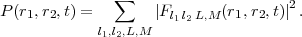(5)

This time-dependent probability density has proved very useful in distinguishing single ionization (where P shows increase with time for only one of r₁ or r₂ large) from double ionization (where P shows increase with time for both of r₁ and r₂ large). However in this probability density function all angular information is lost. This is disadvantageous since many experiments measure ionising electron momenta components parallel to the laser polarisation axis and it is important to make direct comparison with this experimental data [7, 8, 9, 10, 11, 12].

To remedy this deficiency we have written a parallel code (CYLINDRICAL) to calculate the probability density in the z variables, P(z₁,z₂). The z direction turns out to be the most useful in general because in HELIUM the laser light is by convention linearly polarised in the z direction. P(z₁,z₂) is calculated by integrating the wavefunction over ρ_1,2 and ϕ_1,2 (of the cylindrical coordinate system - (ρ, ϕ, z) for each electron), so that, at any given time t:

(6)

where the laser polarisation axis defines the z-axis of each electron. The evolution of this probability density function allows us to distinguish the cases of double ionization in which the 2 electrons are ejected on the same side of the nucleus (z₁ and z₂ have the same sign) from cases of double ionization with the two electrons emerge on opposite sides of the nucleus (z₁ and z₂ have opposite signs). Moreover we can track wavepacket as it makes the transition from one case to the other. Evaluating P(z₁,z₂,t), however, is a significant computational effort - a four dimensional numerical quadrature over (potentially) terrabyte sized arrays spread over tens of thousands of cores.

The program CYLINDRICAL calculates P(z₁,z₂) by numerically evaluating the integral in Equ. 6 for each pair (z₁ and z₂) in a desired range. To do this, the representation of Ψ given in Equ. 1 is substituted into the integral of Equ. 6. The integrand |Ψ(r₁,r₂)|² is expanded in terms of the spherical harmonics that appear in |l₁l₂LM > and the radial variable (r_i) wavefunctions F_l1,l2,L(r₁,r₂) (with M=0). The ϕ variables are easily integrated away, leaving an integral in dρ₁ dρ₂ over an integrand composed of a sum of products of Clebsch-Gordon coefficients, Associated Legendre polynomials, and the F_l1,l2,L(r₁,r₂) functions. The radial variables r_i are related to the cylindrical variables by r_i² = ρ_i² + z_i². Because the integrand is known only at finite-difference grid points that are evenly spaced in the radial variables r_i, the integrand is known only at points that are unevenly spaced in ρ_i. Because of the non-uniform spacings of the ρ_i variables, the integrand is fitted to a cubic spline, which is used to perform the quadrature.

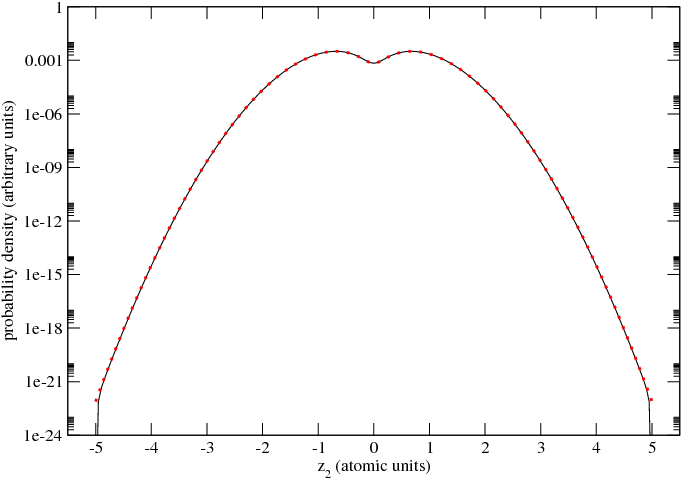
As a test of the new software, we apply it to the following (unnormalised) wavefunction, which resides on partial wave |l₁l₂L >= |1,1,2 >:

(7)

This wavefunction can be integrated analytically using Equ. 6 to obtain the true distribution:

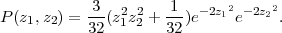(8)

In Fig. 2 we compare the true P(z₁,z₂) (given by Equ. 8) with CYLINDRICAL’s numerical integration of the wavefunction given in Equ. 7. The two methods of calculating P(z₁,z₂) agree to about four significant figures over most of the range of z₂. A discrepancy is only apparent at the end points. At the end points the numerically calculated P(z₁,z₂) (black line) is clamped to zero, whereas the exact result is near 10^-22.

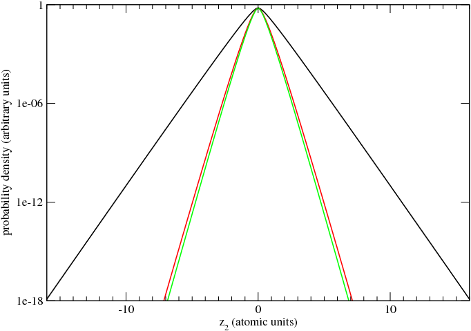
Figure 3 is a logarithmic plot of several probability distributions associated with the ground state of helium. The calculation successfully reproduces the classic features of the helium ground state. The helium ground state Ψ is calculated numerically by HELIUM and transformed to P(z₁,z₂) by program CYLINDRICAL. The ground state Ψ is a linear combination of 6 partial waves. The black line, P(0,z₂), describes the case in which one electron remains near the nucleus (z₁ = 0), while the other spans the full z range of the calculation. The inner electron effectively cancels the positive electric charge of one of the two protons, so that the wavefunction is essentially that of hydrogen asymptotically. The green line, P(z₂,z₂), describes the case in which both electrons are an equal distance from the nucleus, and on the same side of the atom. They see an unscreened nucleus (of two positive charges) and as a result their wavefunction approaches that of the ground state of He⁺. When the two electrons are far from the nucleus simultaneously, but on opposite sides of the atom, then their probability distribution is given by P(-z₂,z₂), the red line. Again, the electrons see an unscreened nucleus of two positive charges, but a more distant negative charge, the other electron, slightly cancels the charge of two protons. The red line is somewhat closer to the hydrogenic (black line) result.

5 Work package 4. Implementation of a new final-state momentum-space code for HELIUM

In work package 4 we proposed a new design and a new implementation of the software that transforms the HELIUM final-state wavefunction from configuration-space to momentum-space. At the time work package 4 was proposed, the original design suffered performance problems, and was limited by the failure of certain MPI collectives (MPI-Gather) on large core counts and large data sets.

The numerical integration generates the wavefunction in configuration-space Ψ(r₁,r₂), but transformation of the wavefunction to momentum-space Ψ(k₁,k₂) can (in the limit in which the Coulomb potentials are negligible) be a convenient and accurate way of calculating the final energy distribution of the electrons for comparison with experiment. This transformation is performed by a 2-dimensional Bessel transformation. In the most recent series of calculations (8000 to 16000 cores on HECToR) the limiting factor on the size and accuracy of the calculation was not the numerical integration itself, but the final-stage Bessel transformation. The problem occurs because the numerical integration operates on a domain localised in r₁ and r₂, but over the full domain of angular momenta, whereas the momentum analysis operates on a domain localised in the angular momenta () but over the full spatial domain. Subsequent to the numerical integration, the wavefunction must be rearranged across the entire machine. In other words, a portion of every single wavefunction on each core must be sent to one or more cores elsewhere on the machine in order to reassemble the wavefunction appropriately. Performed in serial the process is too slow by several orders of magnitude. Performed in parallel by the 8000 cores, the run-time was tolerable, (several hours at most) but the memory limitations of the then current MPI software severely limited the size of wavefunction.

Below we report several successful solutions to the problem. The new software is 4 to 20 times faster than the original software as measured on HECToR (pre-Phase2B). The improvement is due to the superior hardware of the new Phase2B machine, to the use of improved MPI collective routines and to better algorithms. The original proposal was for a fully parallelised solution to the problem. This goal was met through the use of the MPI-alltoallv collective procedure, and this turned out to be the fastest solution on the upgraded HECToR. We report below benchmarks on 8001 cores, along with details of two other useful solutions to the problem.

Work package 4 also called for the implementation of a new transformation of the final state wavefunction using a basis set of Coulomb radial functions (eigenstates of the field-free Coulomb Hamiltonian) rather than a basis set of Bessel functions (which are used in the transformation of the final state wavefunction to momentum space). The two basis sets are identical in the limit in which the Coulomb interaction goes to zero. New software has been written to generate the Coulomb functions as they are needed at run-time. The Coulomb functions are generated by numerically integrating the 1-electron Schrödinger equation with an arbitrary order Taylor series propagator. Surprisingly, the Coulomb functions are generated as quickly as the Bessel functions. The entire transformation, including generation of the basis set functions and projecting them onto the final state wavefunction completes in under 4 minutes in typical medium to large sized problems. We report details of the new software, the test suite, and successful use of the new methods on a significant problem in atom-laser physics that has attracted much attention and controversy recently.

We return now to the problem of rearranging and reassembling the wavefunction across 1000’s of cores on HECToR. To clarify the problem, we describe a specific case. We start with the parameters used in the first benchmark discussed below.

Each core has a local state of 506 partial waves, each of which is a 32 x 32 array of complex numbers called a Block. On 8001 cores this amounts to a 66.3 gigabyte total state. The total memory processed by HELIUM at run-time in this case is  18 times this value, but only the 66.3 gigabyte state is transferred between cores in Stage 1 of the transformation described below.

The problem is to rearrange this data set across the entire set of 8001 cores, and subsequently transform it by writing it on a basis of Bessel or Coulomb functions for energy analysis. This work is done in three stages. On early incarnations of HECToR, attempts to perform this in a single stage failed, evidently due to memory limitations and immature MPI systems software.

The first stage rearranges the data across the 8001 cores. In the original approach to this rearrangement, each of the 8001 cores sends exactly 1 of its 506 blocks to the 1st core, which then assembles all 8001 of them into an array, and writes the array to disk. This is repeated for each of the 506 partial waves.

A second stage is a single core program that reads each of these 3-dimensional arrays from the disk, reassembles the data into a 2-dimensional partial wave, which is them saved to disk.

The third stage transforms the partial waves from configuration space to a representation more suitable for energy analysis of the final-state created by the laser pulse. The third stage will be described in more detail later in this section.

We return to stage 1 and describe new developments and timings on 8001 cores. Three new methods (Methods 2, 3, 4) have been developed that successfully optimise the run-time and solve the poor reliability problems observed on very early versions of HECToR.

Method 1 is the original and simplest method. It was developed to work around failure of the MPI collective routines on the early HECToR, but it was disappointingly slow. The most basic of the MPI procedures, pairs of Send/Recv’s, are used to transfer the data between cores. The Send/Recv pairs are called 8001 times in a loop over partial waves to transfer 8001 blocks to core 0. Core 0 writes this data to disk, and the process is repeated 506 times, once for each partial wave.

Method 2 uses the same Send/Recv loop as method 1, but modifies the 8001 calls to Send/Recv by calling a global synchonization barrier every 1000 iterations through the loop. This produces a surprising and significant improvement in run-time.

Method 3 uses an MPI collective MPI-Gather to perform the operation described above in a single procedure call.

Method 4 (due to Tom Edwards of the Cray Centre for Excellence) uses another MPI collective (MPI-alltoallv), which further parallelises the Input/Output: each of the 506 partial waves is assigned to a core and processed in parallel, so method 4 runs on 506 cores - one for each partial wave.

On test problems of the following size (66.3 gigabyte final-state on 8000 cores) the typical run time of the Send/Recv method on the original (pre-Phase2B) incarnation of HECToR was about 2000 seconds. (A production HELIUM run might use States of 400 gigabyte or greater and run considerably longer.)

Benchmark 1.

8001 cores, 32 x 32 block-size, 506 Partial Waves:

original timings (pre-Phase2B):

1. Send/Recv (original method)     2108 seconds

upgraded HECToR (Phase2B):

1. Send/Recv (original method)     662 seconds

2. Send/Recv (with global barrier)    311 seconds

3. MPI-Gather       242 seconds

4. MPI-alltoallv       102 seconds

Benchmark 2.

8001 cores, 120 x 120 block-size, 55 partial waves:

original timings (pre-Phase2B):

1. Send/Recv (original method)     1715 seconds

upgraded HECToR (Phase2B):

1. Send/Recv (original method)     422 seconds

2. Send/Recv (with global barrier)    390 seconds

3. MPI-Gather       399 seconds

4. MPI-alltoallv       210 seconds

On HECToR method 4, the MPI-alltoallv, is presently the fastest. Unfortunately, this method cannot be used on all machines because it runs on a set of cores equal in number to the number of partial waves. The number of partial waves is very typically in the 500 to 3000 range, so method 4 does not work on the few cores available on a workstation or on clusters of workstations. The MPI-Gather solution (method 3) has the advantage that it runs on the same number of cores as the original numerical integration, so that it will work wherever HELIUM works. In the future it may be desirable to fuse this method to the numerical integration and run as an optional final step. The Send/Recv (with global barrier) is the simplest of MPI procedures, and is the most reliable - we have never seen it fail - and it is often as fast or faster than the MPI-Gather. Because any one of these methods may be the preferred method in a particular limit, the present software offers all four of them. The user chooses the desired method by setting a constant in a parameter module at the start of the program. The chosen method is then called at run-time from a case statement.

Retaining all 4 methods is also of much benefit in the testing process. During testing, the output files of Methods 2-4 are compared with the output of Method 1 in order to verify that the binary outputs of the 4 methods are identical.

We turn now to the problem of generating Coulomb radial functions, and creating a transformation that replaces Bessel functions with both unbound and bound-state Coulomb radial functions. The Coulomb functions - solutions of the Schrödinger equation for one electron in a Coulomb potential - are generated in different ways for the bound and unbound states. In general the Coulomb functions are eigenstates of the finite-difference Hamiltonian, and therefore if highest accuracy is desired they must be calculated on the finite-difference grid with the HELIUM program’s special boundary conditions. This requirement can be relaxed in the case of unbound states. To good approximation the calculation of unbound states can be treated as though we are in continuous space, rather than on a grid of discrete points, and standard methods to perform the numerical integration can be used. On the other hand, very high accuracy in the treatment of the bound states is essential. For example we need to remove from the final state wavefunction the ground state (a bound state with a population of about 0.5) leaving behind the unbound states (the signal we want to analyse) which may have a population of about 10^-7. An error of 1 part in 10⁷ in this case would obliterate the signal we are interested in.

The desired bound states therefore are obtained through a partial eigen-decomposition of the finite-difference Hamiltonian (a large sparse matrix). An iterative Arnoldi-Lanczos method is used to extract from this matrix the first N eigenvectors with the smallest eigenvalues. Typically N is set to 50 - the first 50 lowest energy bound states of the field-free 1-electron singly-ionised helium Hamiltonian are generated and saved to disk. After HELIUM has generated a final-state wavefunction Ψ, all components of Ψ in the direction of these 50 orthogonal bound states are removed.

Originally, the next step was to Fourier transform the wavefunction Ψ(r₁,r₂) to momentum space, by integrating Ψ(r₁,r₂)exp(-ip₁r₁)exp(-ip₂r₂) over d³r₁d³r₂ to get Ψ(p₁,p₂). When this Fourier integration is performed over angular and radial variables, rather than cartesian coordinates, then it becomes an integral in the radial variables over Bessel functions, rather than plane waves.

The new software packages provide Coulomb functions as the preferred (though optional) replacement for the Bessel functions. A public domain package for generating Coulomb functions (using low order Numerov method) was tested but proved to be unreliable and inaccurate. An arbitrary order Taylor’s series integrator was written to replace it. The higher order of the new method enables high accuracy numerical integration without much loss in run-time performance. The Numerov method typically propagated solution of the Schrödinger equation with local truncation errors of order 10^-4. The 10th order Taylor integration gave local truncation errors significantly smaller than 10^-10.

The higher accuracy of the Taylor propagator also makes it easier to detect failure in the integration during the testing process. One of the standard test routines included with the new software generates Coulomb functions from known analytical formulas. Comparison of these results with the numerically integrated results verifies that maximum error in the integrated Coulomb function is of the order 10^-9. Another test routine verifies that the Coulomb functions are orthogonal and have the expected norm.

Asymptotically (at large radial distances r), the Coulomb eigenfunctions and the Bessel functions are identical up to a phase. Testing of the new software includes verification that the Coulomb functions approach the correct values asymptotically.

As a substantial test of the new software, and as a demonstration of the importance of a rigorous quantitative analysis of final-state energy distributions, we have applied the new software suite to a contentious problem that has proved challenging both to theorists and to experimentalists, namely calculation of non-sequential double ionization cross sections in the 2-photon double ionization of helium. Theoretical calculations of these ionization cross sections have yielded predictions that vary in magnitude by a factor of 200: 5 × 10^-54 cm² sec at the low end to 10^-51 cm² sec. We ignore sequential double ionization, a process in which one electron is singly-ionised leaving the other in a bound state of He⁺. Ionization of this residual bound electron at some later time produces a pair of free but uncorrelated electrons. The process of interest to us is the non-sequential one, in which two correlated electrons are freed from the atom and ejected near simultaneously.

To minimise production of sequentially ionised electron pairs the calculation is performed at a relatively low field intensity: 10¹³ W/cm². The pulse in ramped on smoothly over 18 field periods, held constant for 30 field periods, and then ramped to zero intensity over 18 field periods. The numerical integration proceeds for another 30 field periods field-free to allow the doubly-ionised electron pairs to depart the strong coulomb field of the residual ion, and to separate from each other as they do so. Subsequent analysis treats the electrons as though they are non-interacting so that each electron may be regarded as an element of a single-electron dynamical system. This assumption is tested by allowing the electrons to travel an additional 30 field periods field-free, so that their mutual interaction diminishes by a large factor. Recalculation of the physical quantities of interest provides an estimate of sensitivity to mutual interaction.

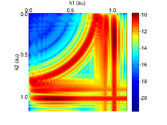
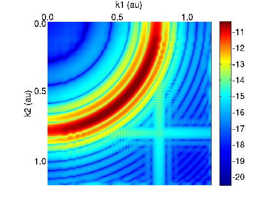
Figure 4 shows the helium atom final state created by the 30 field period laser pulse described above. Plotted is the log of the probability distribution of the two electrons in momentum space, Log (P(k₁,k₂)), where k_i is the magnitude of the i-th electron’s momentum in atomic units (au). P is a probability density, so the probability of finding electrons 1 and 2 with momenta k₁,k₂ in a region of area dk₁dk₂ is P(k₁,k₂)dk₁dk₂. The total kinetic energy K of the two electrons is (in atomic units) K = (k₁² + k₂²) / 2.

The prominent circular arc in Fig. 4 therefore marks a region of constant kinetic energy. The radius of the arc is k = 0.78 au, giving a kinetic energy K = k²/2 = 0.30 au. The laser frequency in atomic units is 1.6 au. (One au is 27.2 eV in energy.) The ground state energy of helium is -2.9037 au, so a 2 photon transition transferring 3.2 au to the 2 electrons should create free electron pairs of total energy 0.30 au, exactly as observed. In this case the total kinetic energy is, within the accuracy of the calculation, equal to the total energy of the electron pair.

The vertical and horizontal bands represent final states in which one of the electrons is bound, and the other ionised. One of the electron is localised in momentum (the unbound electron), and the value of its momentum is largely independent of the momentum of the other electron. This is in contrast to the case described above, in which knowledge of the momentum of the first electron k₁ constrains the momentum of the other electron to k₂ = 2K - k₁²).

The circular arc we identify as non-sequential double ionization. Population in this region represents correlated electron pairs ejected non-sequentially during the laser-atom interaction. The quantity of interest to us in this class of problems is the probability that such an event occurs (for a given laser intensity). The processes is a 2-photon process (two 1.6 au photons are absorbed to ionise the -2.9 au ground state to produce pairs of free electrons of total energy 0.3 au). It follows that the probability scales as the square of the intensity. The ionization cross section for this process is proportional to the probability divided by the intensity squared, since we are in a perturbative regime. The cross section is especially useful because it is intensity independent.

When the cross section is calculated (by integrating P(k₁,k₂) over the circular arc to obtain the probability all events occurring it this region of momentum space) we discover why the calculation has proved difficult. There is no natural division between the arc and the linear features that represent bound states. The calculated probability can vary by a factor of 2 or more depending on the choice of boundary between arc and band. In momentum space (Fig. 4) it appears that the two features - the arc representing non-sequential double ionization and the bands representing bound states - are fused.

From the data displayed in Fig. 4 we cannot reliably calculate the double-ionization cross section, (which is proportional to population in the circular arc), but with the new software introduced in this section we have been able to develop 3 methods of calculating the desired quantity with good quantitative accuracy. The 3 methods of analysis independently give the same answers to within 2 percent.

The first of these methods is performed using the momentum space approach described above, but with a single pre-processing stage in which all bound states (up to principal quantum number 9) of the residual He⁺ ion are removed. The bound states are eigenstates of the hydrogenic He⁺ ion on the finite-difference grid, calculated using the same boundary conditions used during the numerical integration performed by HELIUM on an identical finite-difference grid. 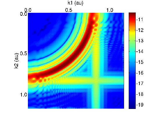The bound states are calculated in advance using an Arnoldi eigen-decomposition, and stored in an external file. Figure 5 shows the helium final state in momentum space with these bound states removed. All that remains is the desired circular arc. Integration over the probability density function in the arc yields the desired physical quantity: probability of non-sequential double ionization.

The second approach to this problem is the more satisfactory in general, because it decomposes the helium final state into a linear combination of states that are eigenstates of the field-free helium Hamiltonian (in the limit in which the two final state electrons are non-interacting). This new basis of eigenstates, which we call Coulomb states, differs subtly from the basis set used to construct the momentum space final state shown in Fig. 4. In fact the Coulomb states are identical to the momentum space states in the region of space in which the Coulomb potential can be neglected, which is generally the case in this problem. This asymptotic equality between the basis sets is used as part of the software’s test suite. Unfortunately, the difficulty described above, in which unbound states appear fused to the bound states, occurs in the region of space in which the Coulomb potential is non-negligible. The use of Coulomb states solves this problem. In the Coulomb basis we are able to resolve the bound and the unbound states. 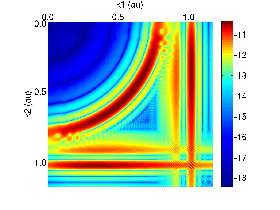As a result, in the Coulomb basis it is not necessary to remove bound states from the final state prior to analysis. This was an unexpected result. Figure 6 shows final state written on a basis of Coulomb states. Clear space now separates the circular arc from the bound state that caused the difficulties described above. Calculation of the probability of non-sequential double ionization (integration of P(k₁,k₂) over the arc) yields the same answer as the momentum space calculation (Fig. 4).

Finally, in Fig. 7 we show the final state in Coulomb space with bound states removed. Comparison with the momentum space calculation (Fig. 5) shows only subtle differences. Non-sequential double ionization probabilities obtained from the data of Fig. 7 agree with the previous calculations.

Acknowledgements:

This project was funded under the HECToR Distributed Computational Science and Engineering (CSE) Service operated by NAG Ltd. HECToR - A Research Councils UK High End Computing Service - is the UK’s national supercomputing service, managed by EPSRC on behalf of the participating Research Councils. Its mission is to support capability science and engineering in UK academia. The HECToR supercomputers are managed by UoE HPCx Ltd and the CSE Support Service is provided by NAG Ltd.

References