Next: Outcome Up: Improving Load Balancing and Previous: Flredcomp
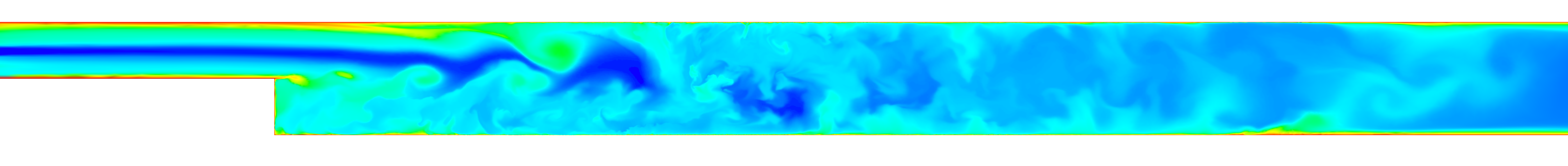
A single benchmark case was tested which represent a common use-case for Fluidity simulations. This is a backward-facing step CFD example (Fig. 4) on a piecewise-linear continuous Galerkin discretisation (P1P1). This discretisation is a common choice for CFD applications and also allows comparisons to Sam as a baseline. Other benchmark cases were either not adaptive, or if made adaptive, could not be performed using Sam.
 |
 |
It was unfortunately not possible to use ParMETIS through Zoltan on HECToR for any of the profiling runs. This had previously been possible on HECToR but at the time the profiling runs were conducted there appeared to be a bug in Zoltan 3.5. Runs using ParMETIS through Zoltan failed due to requiring an extra callback which according to the Zoltan documentation should not be needed. This issue has been raised with the Zoltan developers. The code has previously been run on HECToR and other systems using ParMETIS through Zoltan 3.4 so this issue should be resolved in the near future.
It was also not possible to conduct profiling runs on HECToR which used PT-Scotch through Zoltan on more than 16 processes. This appears to be a problem with PT-Scotch which gives an MPI error when running on more than one core of the HECToR system. This issue has been raised as a bug on HECToR system.
The profiling results presented below are from runs on the HECToR Phase 3 system. The Phase 3 system is a Cray XE6 system, offering a total of 2816 XE6 compute nodes. Each compute node contains two AMD 2.3 GHz 16-core processors giving a total of 90,112 cores - a theoretical peak performance of over 800 Tflops. There is presently 32 GB of main memory available per node, which is shared between its thirty-two cores, the total memory is 90 TB. The processors are connected with a high-bandwidth interconnect using Cray Gemini communication chips. The Gemini chips are arranged on a 3 dimensional torus. Further profiling work on the Phase 3 system of the other test cases was not possible due to time constraints.
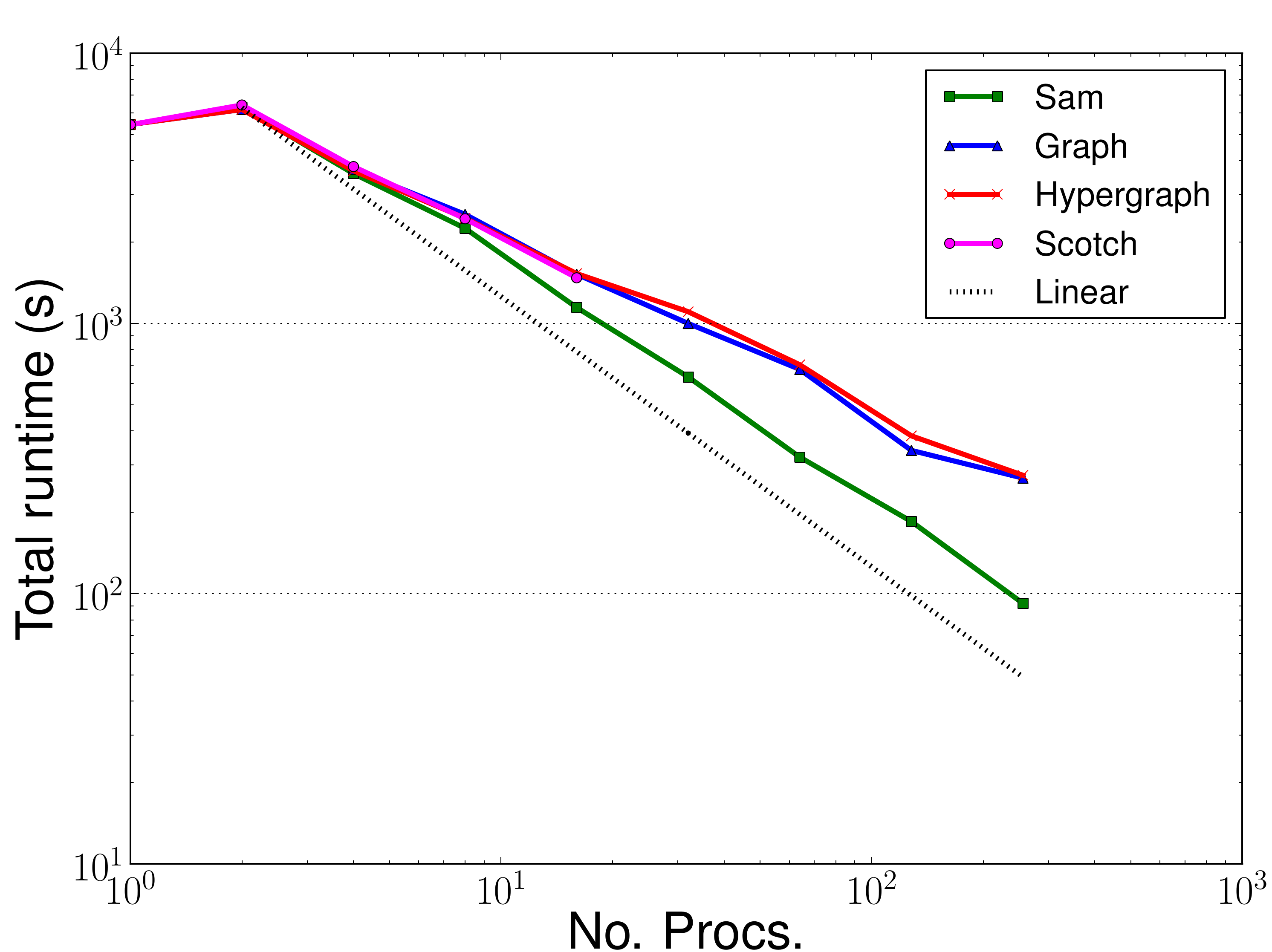
Figures 5 through 10 above show the profiling results for the small backward-facing step benchmark run on HECToR. This is a small benchmark which uses approximately 23,000 elements that is typically run on 32-64 processes. Here it has been run on up to 256 processes to test the different partitioners. In addition, dynamic adaptivity of the mesh was performed every two timesteps, rather than the usual 10 to 20. As such, the adaptive algorithm dominates the runtime of these benchmarks. In most problems this would not be the case and instead the assemble and solve phases would dominate the total runtime.
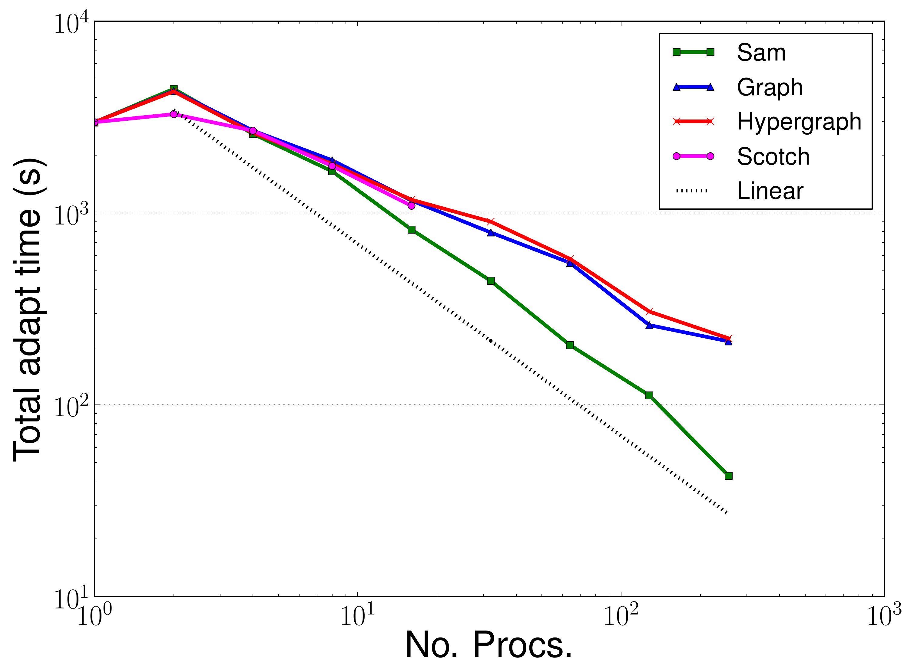 |
Figure 5 show the performance of the Zoltan implementation matching the Sam performance up to 8
processes. At ![]() 8 processes the overall runtime for Zoltan becomes greater than that for Sam. This is due to
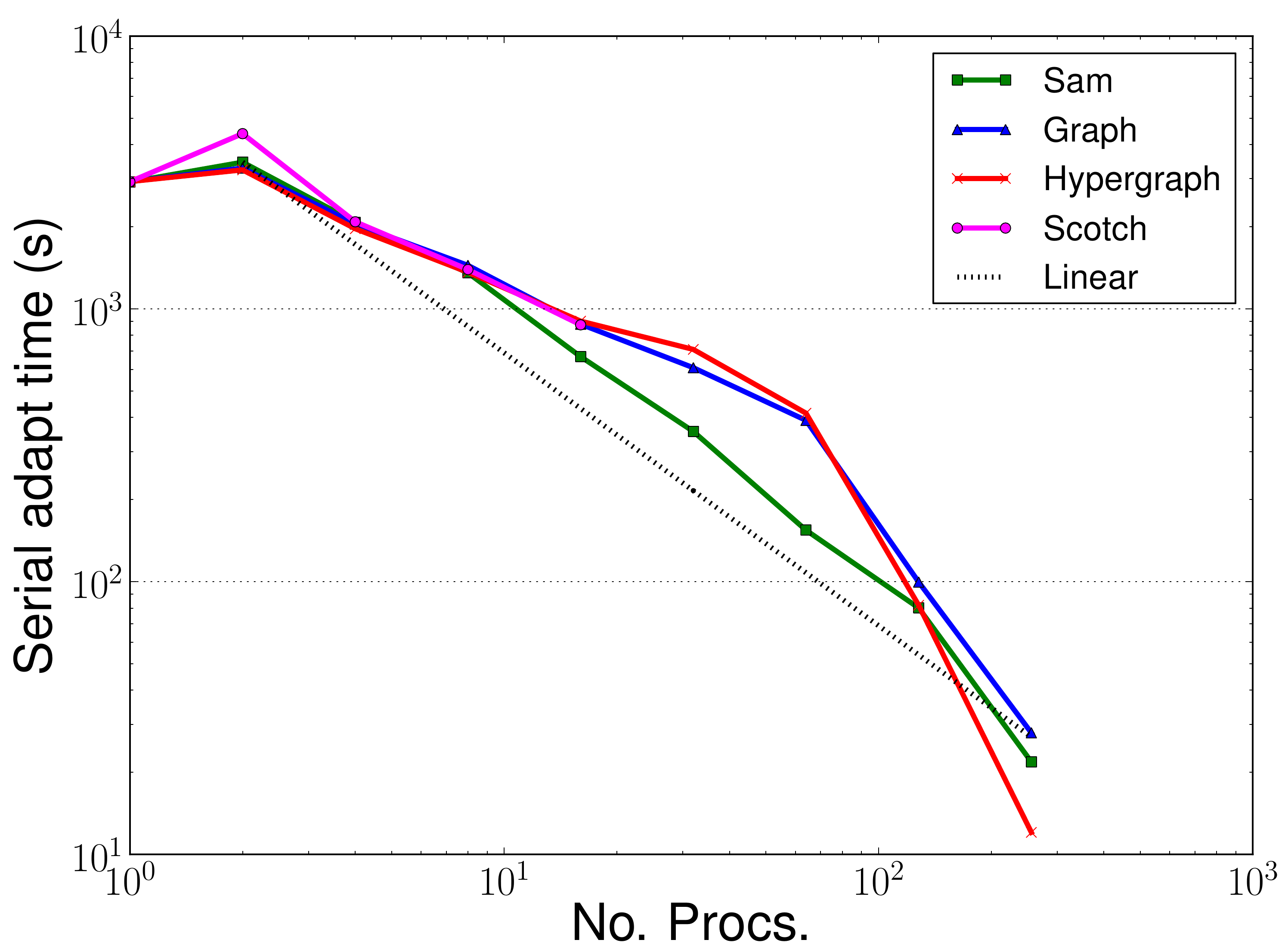
the increased adapt time when using Zoltan (Fig. 6). It was expected that the time to complete the adapt phase in Zoltan may be
longer than in Sam due to Zoltan being a general purpose solution. Sam only works for particular element
types which allow the field data to be migrated at the same time as the nodes. The Zoltan solution requires
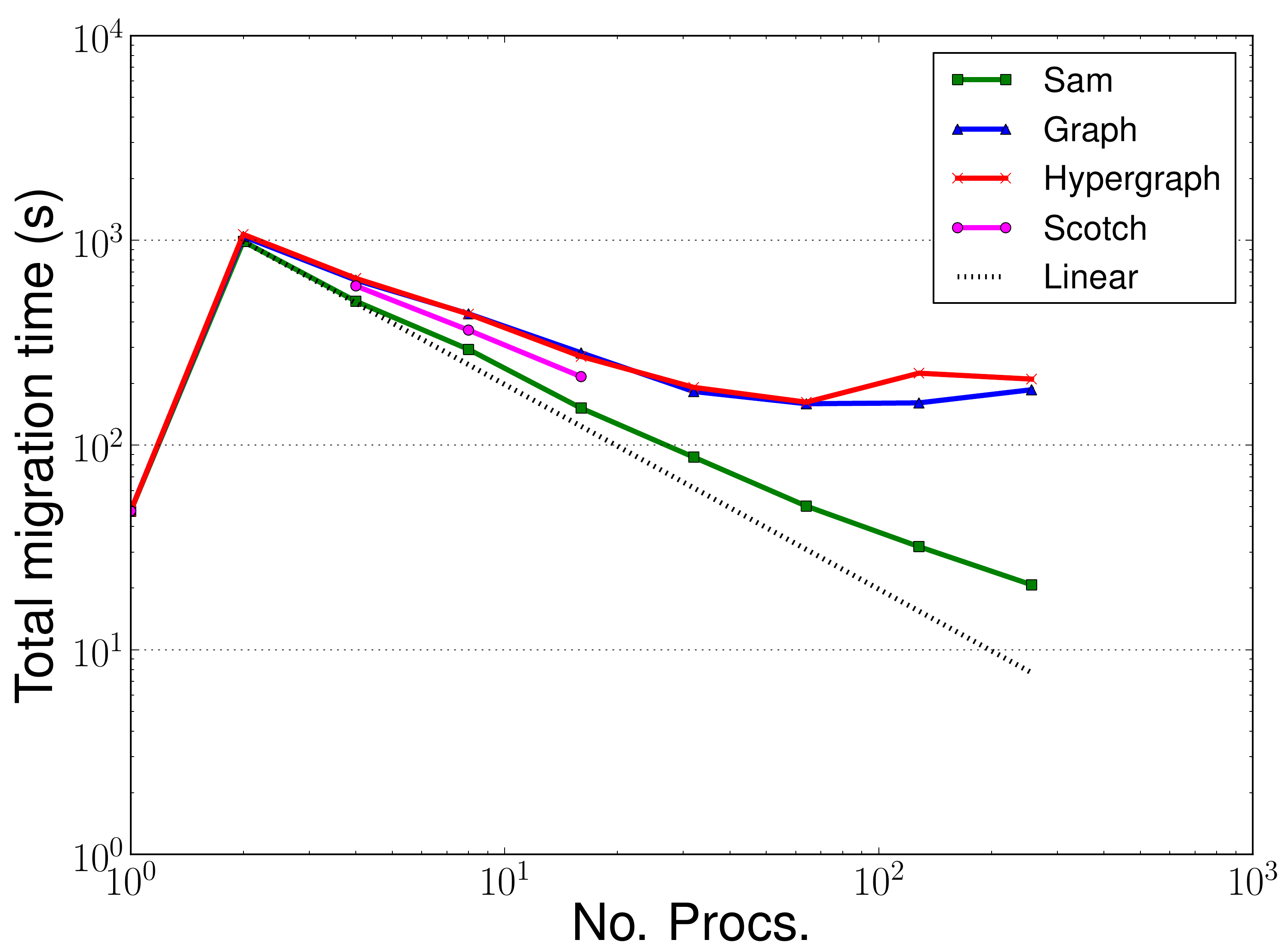
an extra migration phase to migrate the fields data separately. Figure 10 show that the extra migration
only impacts the Zoltan performance when the partitioner is being worked heavily, as happens when you have a
small problem being divided up on to too many processes. The same increase is not seen in the serial adapt times
(Fig. 9).
8 processes the overall runtime for Zoltan becomes greater than that for Sam. This is due to
the increased adapt time when using Zoltan (Fig. 6). It was expected that the time to complete the adapt phase in Zoltan may be
longer than in Sam due to Zoltan being a general purpose solution. Sam only works for particular element
types which allow the field data to be migrated at the same time as the nodes. The Zoltan solution requires
an extra migration phase to migrate the fields data separately. Figure 10 show that the extra migration
only impacts the Zoltan performance when the partitioner is being worked heavily, as happens when you have a
small problem being divided up on to too many processes. The same increase is not seen in the serial adapt times
(Fig. 9).
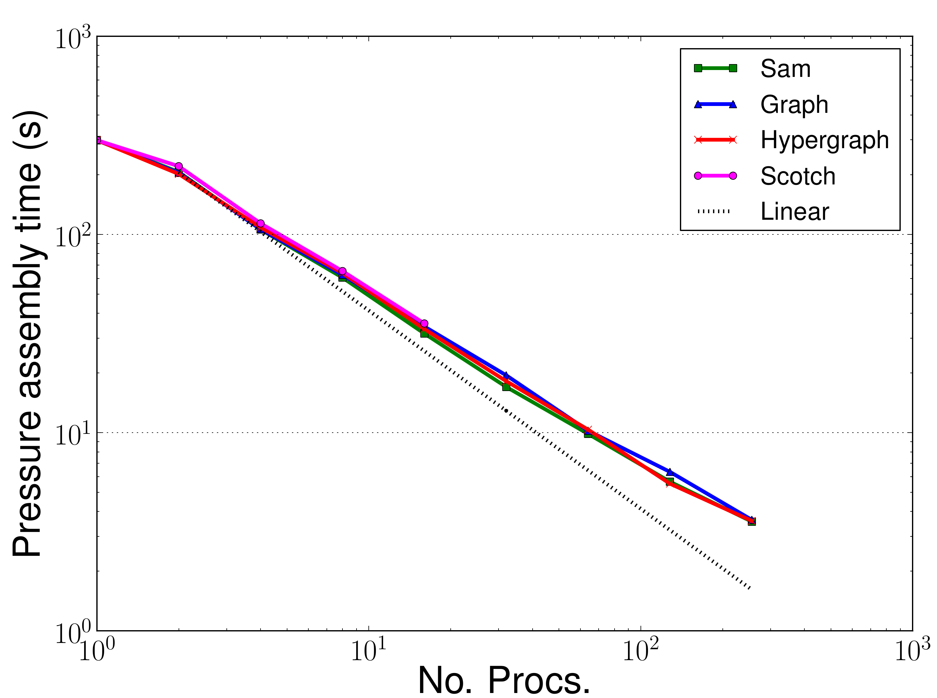
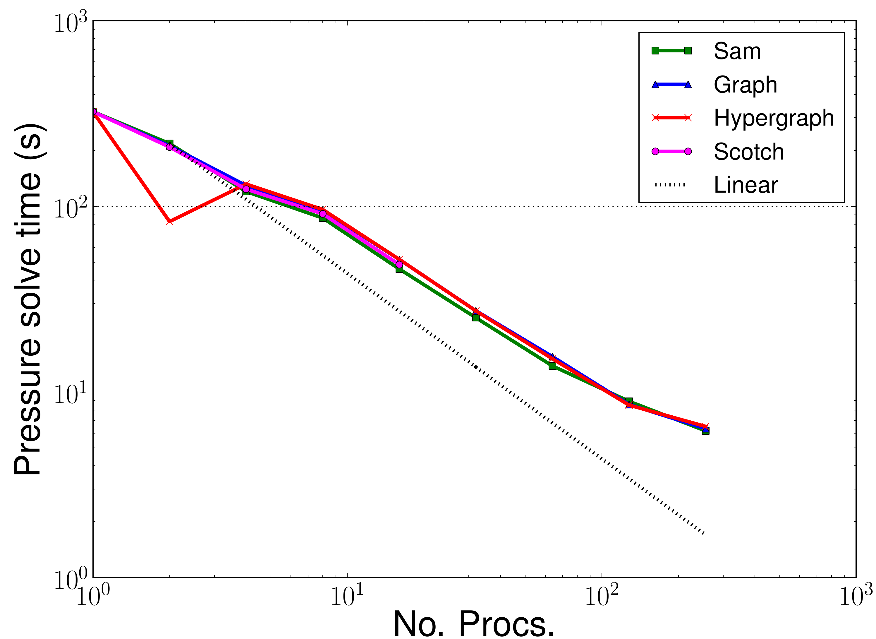
The hope was that the access to different partitioners, particularly the hypergraph partitioner, would improve the load balance for the assemble and solve phases and these sections would hence see a performance improvement. As can be seen from Figures 7 and 8 there has been no performance improvement in the assemble or solve phases.
Jon Hill 2012-03-02