|
|
Summary of the Project Progress
During the course of this project dCSE Fluidity-ICOM has been transformed from a code that was primarily used on institution level clusters with typically 64 tasks used per simulation into a highly performing scalable code which can be run efficiently on 4096 cores of the current HECToR hardware (Cray XT4 Phase2a). Fluidity-ICOM has been parallelised with MPI and optimised for HECToR alongside continual in-depth performance analysis.
The following list highlights the major developments:
Extensive profiling has been performed with several benchmark test cases using CrayPAT and VampirTrace:
The Fluidity-ICOM (Imperial College Ocean Model 1 ) dCSE project commenced on 1st July 2009 and is scheduled to end on the 31st May 2010. The principal investigator on the grant was Mike Ashworth from the Advance Research Computing Group (ARC), Science and Technology Facilities Council (STFC). This highly collaborative project also involved Gerard Gorman, Matthew Piggott Stephan Kramer from Applied Modelling and Computation Group (AMCG), Imperial College London.
The Fluidity-ICOM dCSE project comprised of three work packages (referred to as WP1, WP2 and WP3), WP1 concerned with profiling and optimisation, WP2 concerned with scalability of mesh adaptivity and WP3 concerned with parallel I/O. The overall aim of this work is to develop Fluidity-ICOM from being a state-of-art workstation and cluster based code to become a model able to run efficiently on the largest supercomputing platforms, which will also help Fluidity-ICOM make the transition from local research software to being high quality community software.
Fluidity-ICOM is build on top of Fluidity, an adaptive unstructured finite element code for computational fluid dynamics. It consists of a three-dimensional non-hydrostatic parallel multiscale ocean model, which implements various finite element and finite volume discretisation methods on unstructured anisotropic adaptive meshes so that a very wide range of coupled solution structures may be accurately and efficiently represented in a single numerical simulation without the need for nested grids (Ford et al., 2004; Pain et al., 2005; Gorman et al., 2006).
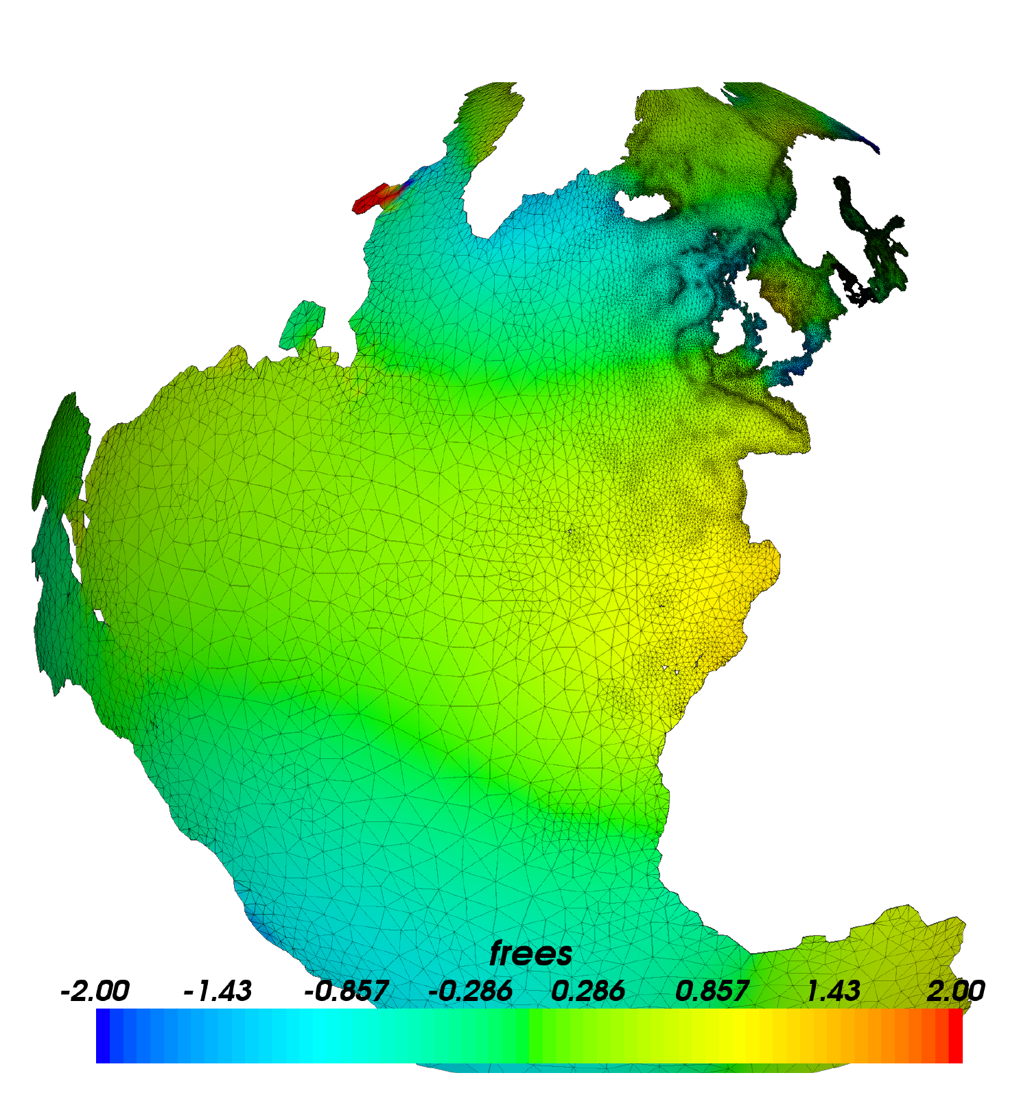
Developing an unstructured mesh ocean model is significantly more complex than traditional finite difference models. Apart from the numerical core of the model, significant effort is also required to develop pre- and post-processing tools as there are no standards yet established within the community. For example, initial mesh generation must confirm to complex bathymetry and coastlines, which exerts a critical influence over the dynamics of the ocean. In practice, there is a trade-off between how close the discretised domain is to reality, and how appropriate it is for numerical simulation with limited computational resource. To achieve this, specialised mesh generators such as Terreno (Gorman et al., 2008) have been developed as the geometries do not lend themselves to standard packages which use CAD models. A typical bathymetry conforming unstructured mesh is presented in Figure 1.
Fluidity-ICOM can also optimise the numerical mesh to control modelling error estimates using anisotropic mesh adaptivity. Large load imbalances are to be expected following the mesh adaptivity, therefore dynamic load-balancing is required. When re-balancing the mesh a combination of diffusion repartitioning, and clean parallel repartitioning with domain remapping, is used to minimise data migration. While this is currently done using a combination of ParMETIS and a bespoke code for data migration (see (Gorman et al., 2009)), work is being done on integrating Zoltan 2 instead.
Solving sparse linear equations is one of the most time consuming parts in Fluidity-ICOM. For systems of equations with low/moderate condition number, Fluidity-ICOM uses standard preconditioners and solvers from PETSc 3 . When the condition number is high Fluidity-ICOM use an AMG preconditioner designed specifically for ocean problems which outperforms all conventional preconditioners and black box AMG preconditions tested (e.g. Prometheus and HYPRE/BoomerAMG). However, attention must always be paid to the scaling as the coarsening typical process of AMG makes scaling more difficult.
Fluidity-ICOM uses state-of-the-art and standardised 3rd party software components whenever possible. For example, PETSc is used for solving sparse linear systems while Zoltan is used for many critical parallel data-management services both of which have compatible open source licenses. Python is widely used within Fluidity-ICOM at run time for user-defined functions and for diagnostic tools and problem setup. It requires in total about 17 other third party software packages and use three languages (Fortran, C++, Python).
Fluidity-ICOM has a relatively complex set of dependencies. In order to aid developers and users that want to build the code on HECToR environment modules have been created to set up both production builds of the code together with more specialised ones for profiling with CrayPAT and Vampir. Details can be found on AMCG wiki page 4 .
There are two main software environment for which modules are developed on HECToR software for Fluidity-ICOM: GNU and PGI. Several software environment issues were encountered during the course of the project (see Appendix A.A).
As part of the dCSE Fluidity-ICOM project, a set of HPC benchmarks has been set up which well characterise the performance of the code for a wide number of applications. This allows us to:
This standardised set of benchmarks is also used by other HPC collaborative projects which ran concurrently to this work, namely those with Fujitsu and the NAG group. One is also funded through distributed Computational Science and Engineering (dCSE) Support awards from HECToR (High-End Computing Terascale Resource), the UK national supercomputing service . This helped enhance the level of collaboration across the different projects.
The benchmark configurations were created by running the model for an initial spin up time, in order to allow transient dynamics associated with initialisation to die down, and then checkpointed. The benchmark then consists of running the problem, restarting from the checkpoint, only for a few time steps. The rationale behind this approach is to ensure the time steps performed during the benchmark are representative of the overall run; time steps in the initial period can behave very differently due to the model having to adjust to physics imposed and spurious dynamics having to die out first.When configured in this way benchmarks only need to be run for a few number of time steps before reliable profiling results are generated.
For some benchmarks, the initial spin up time can be quite long, for example 1 year of simulation time for the gyre. The spin up runs are therefore run on a moderate number of processes, typically 64. Because each process reads and writes its own partition, the resulting checkpoint will already be decomposed into 64 subdomains. The program flredecomp, from the Fluidity-ICOM tool kit, can then be used to repartition the problem into different number of subdomains, so that strong scaling analysis can be performed. As per usual in strong scaling analysis, the range of partitions numbers is restricted by the overall problem size. Too many processors for a given problem leads to excessive communication costs relative to computation costs due to the size of the mesh halo approaching the size of the subdomain. With a small number of processes the problem might become too big to fit in memory. For this reason some of the benchmarks are provided in different resolutions, giving a different total number of degrees of freedom, and scaling is measured relative to the lowest number of processes that the problem could be run on.
Available configurations are:
For each of the benchmarks a report has been written, giving a more detailed description of both the physical setup and the numerical configuration. The results of the profiling analysis described below is analysed in greater detail for each of the benchmarks in these reports.
The wind-driven baroclinic gyre benchmark is used for the solver comparisons and
scalability analysis. A gyre in oceanography is a large system of rotating ocean
currents, particularly those involved with large wind movements. The flow is
dominated by a balance in the horizontal between the Coriolis force and the free
surface gradient. In a baroclinic gyre a density stratification, typical for the ocean
domain, is taken into account. The equations used by Fluidity-ICOM to model this
configuration are the 3D non-hydrostatic Boussinesq equations. In a domain
V ⊂  3 these take the form:
 + 2Ω ×u-∇⋅ + 2Ω ×u-∇⋅ |  + + | (1a) |
| + ∇p | = fwind + ρgk, | (1b) |
| ∇⋅u | = 0, | (1c) |
 -∇⋅ -∇⋅ | = 0, | (1d) |
| ρ | ≡ ρ(T), | (1e) |
where D∕Dt = ∂∕∂t +  ⋅
⋅ is the total derivative, p is the perturbation pressure, g
is the acceleration due to gravity, ρ is the perturbation density and fwind is the
wind forcing term. Rotation of the earth is taken into account via the vector
Ω = (0, 0,f)T , where f = f
0 + βy, the so called beta-plane approximation. T is
the temperature, but additional scalar fields such as salinity and tracers
can be dealt with analogously, in which case they may be included in the
equation of state (1d). A diagonal viscosity tensor ν is used to represent
(effective) stresses in the model. κT is the thermal diffusivity tensor, also
assumed to be diagonal. No turbulence models have been applied in this
benchmark.
is the total derivative, p is the perturbation pressure, g
is the acceleration due to gravity, ρ is the perturbation density and fwind is the
wind forcing term. Rotation of the earth is taken into account via the vector
Ω = (0, 0,f)T , where f = f
0 + βy, the so called beta-plane approximation. T is
the temperature, but additional scalar fields such as salinity and tracers
can be dealt with analogously, in which case they may be included in the
equation of state (1d). A diagonal viscosity tensor ν is used to represent
(effective) stresses in the model. κT is the thermal diffusivity tensor, also
assumed to be diagonal. No turbulence models have been applied in this
benchmark.
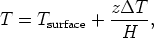
A linear stratification has been used as an initial condition for the temperature:
 | (2) |
with a surface temperature of Tsurface = 20 and a temperature difference ΔT = 10. The vertical coordinate z is chosen such that z = 0 at the surface and z = -H = -2000 m at the bottom. A simple linearised equation of state is used:
 | (3) |
where α = 2.0 × 10⁻⁴ K-1 is the thermal expansion coefficient, and T 0 = 10.
The wind forcing, fwind, is applied as a stress integrated over the surface, given as the analytical function:
 | (4) |
The domain extends from x = 0 to x = Lx = 1000 km and y = 0 to y = Ly = 1000 km. This simulates a mid-latitude double gyre, with easterly winds in the north and south, and westerly wind in the middle of the domain. The amplitude of the wind stress is τ0 = 0.1 Nm-2.
The Boussinesq equations (1a) and (1b) are discretised via a finite element integration using a P1DG - P2 velocity, pressure element pair. This element pair has a number of advantageous properties for ocean simulations, a.o. its beneficial balance properties (Cotter et al., 2009). The incompressibility constraint (1b) is enforced through a pressure correction approach. The non-linearity in the advection terms, and the coupling of the heat equation and the buoyancy term are dealt with in a Picard iteration. The free surface is solved in conjunction with the pressure equation. Finally the heat advection diffusion equation is solved with a standard P1 SUPG discretisation (Gresho and Sani, 1998).
The mesh used in the baroclinic gyre benchmark test case has 10 million vertices; resulting in 200 million degrees of freedom for velocity due to the use of DG.
Fluidity-ICOM uses the PETSc library for the solution of the sparse linear systems arising from the numerical discretisation. A wrapper petsc_solve takes in the CSR matrix, and constructs a PETSc matrix data type, sets the solver and preconditioner options, and then passes the system to PETSc to solve. This wrapper offers full access to several classic algorithms contained in PETSc and also get the extra benefits with new added algorithms without extra work.
For the gyre test case, the pressure matrix has a very high condition number, making it very difficult to solve using conventional preconditioners and solvers. Here we use an AMG preconditioner which is the best choice for large systems (because of their better scaling properties), and ill-conditioned systems, such as those in large aspect ratio problems, or more generally problems in which there is a large variety in length scales. An algebraic multigrid method targeted specifically at large aspect ratio ocean problems is developed for the Fluidity-ICOM model (Kramer et al., 2010). This multigrid method is applied as a preconditioner within a Conjugate Gradient iterative method.
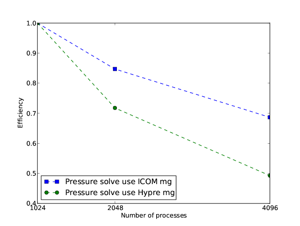
PETSc also provides an interface to other AMG methods such as BoomerAMG in HYPRE 5 . The parallel efficiency for the pressure solver using Fluidity-ICOM MG and BoomerAMG preconditioners are in Figure 2. We can see Fluidity-ICOM MG has better scalability than BoomerAMG.
|
|
There were several major updates for matrix assembly, Fluidity-ICOM now supports block-CSR for the assembly and solves of vector fields and DG fields.
Applied sparse matrix reordering schemes for generating narrow-banded (or clustered) nonzero patterns via the PETSc interface.
Users should not spend time optimising a code until after having determined where it spends the bulk of its time on realistically sized problems. Profiling is the best way to address both the serial execution of the code(such as cache usage, vectorisation) and parallel aspects, such as parallel efficiency, load balancing and communications overheads. Profiling using CrayPAT and Vampir on HECToR has been performed on the gyre benchmark test case which is of particular relevance to GFD applications. CrayPAT and Vampir are the two main tools being used for Fluidity-ICOM profiling.
In theory, the process for using profiling tools like CrayPAT and Vampir would consist of firstly running a representative benchmark test case with tracing enabled to produce trace files, then viewing the tracing data using specialised tools. However, in the case of large benchmark test cases this may not be possible. Even for a relatively small Fluidity-ICOM dataset of 0.21 million nodes, with CrayPAT suggested automatic profiling options, trace files can be hundreds of GBytes which makes analysis impossible. The size of the trace file data depends on the nature and intensity of the profiling experiment and the duration of the program run. Using runtime variables such as PAT_RT_SUMMARY in CrayPAT could make a big reduction of data size but at the cost of fine-grain details. Specifically, when running tracing experiments, the formal parameter values, function return values, and call stack information are not saved. Determining a way to control profiling data size whilst at the same time gathering in-depth and informative data is key for understanding the performance bottlenecks in large realistically sized problems. Under such circumstances, a starting point is to use simple timing hooks in the code to get a coarse grain profile of code performance, then to use these results as a basis for more fine grain profiling with the CrayPAT/Vampir API in the identified areas of interest.
Following the above procedure, a timing module for coarse level profiling of the code was added (r12743), The target of this work is to analyse Fluidity-ICOM on a large number of processes (cores) with the gyre test case. The number of processes ranges from 1024 to 4096. In order to identify the issues for this scale of processes, the 10 million node mesh has been generated. During the profiling, several major issues were resolved:
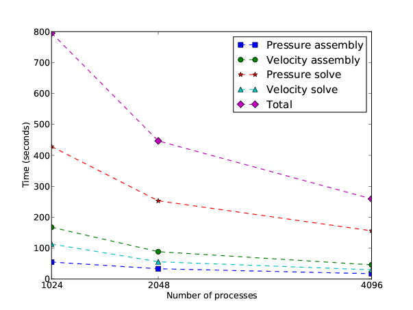
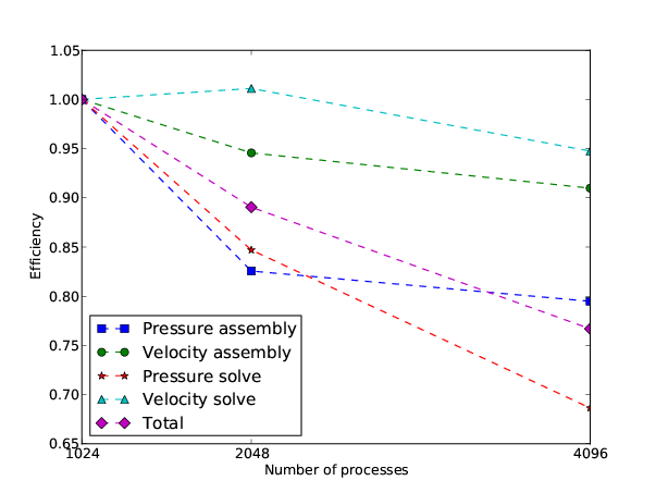
We focus on the solution of the momentum equation (1a) in combination with the incompressibility constraint given by the continuity equation (1b), as this is by far the main cost of the simulation, and dominates the overall scaling of the simulation. The solution process consists of the assembly of the linear systems representing the discretised momentum equation and the pressure equation, and the solution of those. Thus the scaling analysis of the momentum equation is naturally broken down into 4 parts: assembly of the pressure matrix, linear solve for the pressure equation, assembly of the discretised momentum (velocity) equation, and linear solve of the momentum (velocity) equation.
From Figure 3, we can see that matrix assembly for pressure and velocity can take more than 30% of the total simulation time with 1024 cores, where the pressure solver occupies nearly 53.9% of the total simulation time. The matrix assembly phase is expensive for a number of reasons, including: significant loop nesting, where the innermost loop increases in size with increasing quadrature; indirect addressing (due to unstructured meshes) and cache re-use.
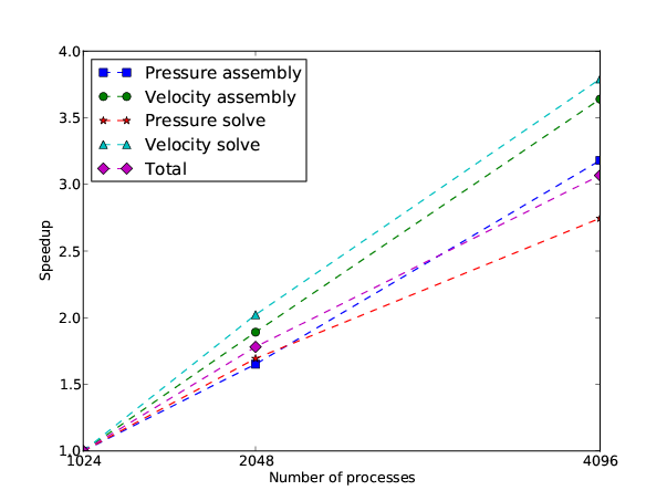
Comparing with 1024 cores, Figure 4 and Figure 5 show the speedup and efficiency of momentum solver and each of its components. As we can see from the graphs, the scaling is very respectable. Velocity is being solved using a discontinuous Galerkin method (DG). This is showing very good scaling characteristics.
The pressure assembly is showing less parallel efficiency than the velocity assembly. It is to be noted that this assembly only occurs once in an entire model run, so is expected to take only a small fraction of runtime in a normal run with significantly more time steps. Due to non-linearities, the momentum equation does have to be re-assembled every non-linear iteration within a time step.
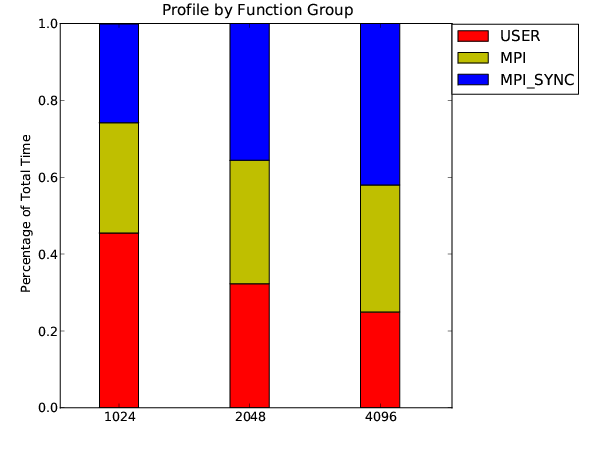
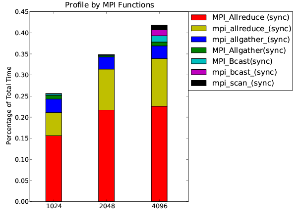
Using CrayPAT, we obtained the statistics of three groups of functions, namely MPI functions, USER functions and MPI_SYNC functions. MPI_SYNC is used in the trace wrapper for each collective subroutine to measure the time spent waiting at the barrier call before entering the subroutine. Therefore, MPI_SYNC statistics can be a good indication of load imbalance. The time percentage of each group is shown in the Figure 6.
With core counts from 1024 to 4096, we can see that the time percentage spent in MPI increases from 28.7% to 33.1% while USER functions drop from 45.5% to 24.9%, and time percentage of MPI_SYNC increase from 25.7% to 42.0%. This lead us to identify the top time consuming functions in each group along with their calling hierarchy.
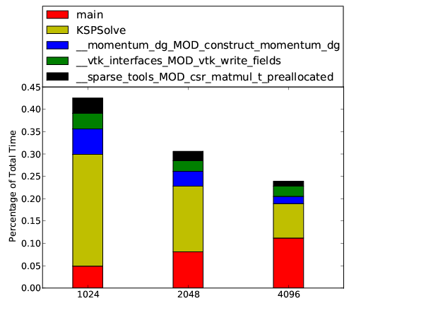
Figures 7-9 give the top time consuming functions in each group. In Figure 7, the speed up of the linear solver KSPSolve is about 3.5 with 4096 cores comparing with 1024 cores according to the CrayPAT tracing results. The function main represents the functions that have not been traced in the code. These functions are outside of momentum solver. Future work will focus on these functions with poor scaling behaviour.
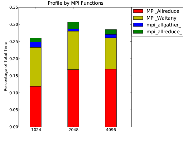
The most time consuming of the MPI groups is MPI_Allreduce. It is expected that this collective operation does not scale well. However on the XT4 the scaling is relatively good from 2048 to 4096 cores in Figure 8. From the call tree generated by CrayPAT, it becomes clear that this function is called from PetscMaxSum within PETSc. MPI_Waitany is indicative of the quality of the load balancing. Given that this amount does not increase significantly between runs on 1024 to 4096 cores in Figure 9, it does not appear that load-balancing is worsening noticeably as the core count increases.
In Figure 9, MPI_Allreduce accounts the most part of waiting time spent in the barrier, it is worth to check if it is possible to combine several MPI_Allreduces together. MPI_Bcast and MPI_SCAN are becoming more significant on 4096 cores, compared to runs on 1024 and 2048 cores.
As Fluidity-ICOM makes extensive use of third party software, it is also important to obtain insight in performance issues from these other software packages.
Profilers like CrayPAT and Vampir normally require direct access to the source file or the object file, which are typically not available for third party package software installed on a given system. This will limit the view on the overall performance of applications widely using such software packages. For instance, Fluidity-ICOM uses PETSc as the sparse linear system solver. With nearly 70% time spent inside PETSc, it is necessary to understand the performance profile within PETSc as this generally dominates the overall performance of Fluidity-ICOM. However without direct access to the source and object file, it is very hard to trace the specific functions in PETSc. One possible solution is to rebuild and install PETSc in the user home directory. In this case CrayPAT can profile PETSc as normal USER functions.
A problem will then be how to properly reduce the profiling data from PETSc as there are very many different PETSc functions, called from various places. This will generate a large amount of profiling data. Using the API functions of profiling tools may be a solution but it will require recompiling PETSc each time a different grouping is chosen. Another choice is to generate a specific function list which is a subset of PETSc functions. Directly instrumenting the subset of PETSc functions can also help to reduce the amount of profiling data and obtain useful statistics.
Adaptive mesh methods aim to produce a mesh which achieves a user specified error among the computational domain; often with user specified constraints on mesh edge lengths, problem size, geometry and mesh gradation. This approach to error control can also be viewed as optimising the computational efficiency of a simulation; reducing time to solution and even resolving solution features that might have otherwise been impractical to compute using a static mesh on a given computer.
Adaptive methods must be coupled with parallel methods for many problems of practical interest. The mesh optimisation method is described in detail by (Pain et al., 2001). The main challenges associated with parallel mesh optimisation, include:
Generally, an adaptation involves a change in the local mesh configuration. If any mesh entity is to be adapted then all domains that contain information specific to that entity must also be updated. Unlike hierarchical mesh refinement methods (e.g. Jimack (1998)), the very nature of the mesh optimisation method used precludes the independent prediction on different processes of the local connectivity of the final mesh.
A reasonable estimate of the relative computational load per process can be obtained from the number of mesh vertices assigned to the partition on that process, as that defines the size of the linear systems to be assembled and solved. At the outset of the parallel simulation, graph partitioning is used to define a domain decomposition that balances the number of nodes per process and thus provides an even distribution of work throughout the processes. However, mesh optimisation operations such as edge-collapsing (node deletion) and edge-splitting (node insertion) disrupt this balance. The induced load-imbalance can range from just a few percent to many orders of magnitude in difference. Because of this, graph repartitioning and data migration (e.g. the redistribution of mesh entities across processes in order to satisfy a new graph partitioning) are key components for parallel mesh optimisation. This operation adds further computational and communication overheads to mesh adaptivity.
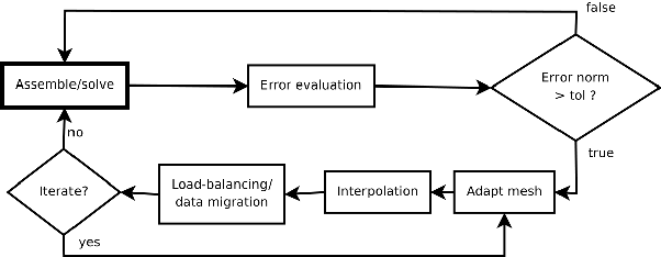
A description of the algorithm, illustrated in figure 10, is now summarised. Firstly, the serial mesh optimisation method is applied to each sub-domain independently with the constraint that no mesh elements on a partition may modified. Once the adaptive algorithm terminates, load-imbalances will in general have arisen due to the local refinement and coarsening of the mesh. This motivates a re-partitioning of the domain. The error metric field can be used to predict the local density of elements after optimisation (Pain et al., 2001). This allows us to define suitable node-weights for the graph partitioning method to be used in calculating a well-balanced partition. After applying mesh adaptivity this should be close to unity everywhere except at domain partitions where mesh adaption was explicitly disabled. In addition, edge-weights are defined which are proportional to the error metric. High weights correspond to elements whose error metric indicate that they will be targeted by the adaptive mesh algorithm; mesh regions through which we wish to strongly discourage a mesh partition. This choice of edge weight, when used with diffusive repartitioning methods, has the effect of perturbing partitions away from elements that require further optimisation while still balancing the load. Mesh adaptivity is then reapplied to the mesh to address any sub-optimal elements. The procedure is then repeated if necessary. It is clear that repartitioning is required to address the load-imbalance caused by mesh adaptivity; the computational cost of this load-balancing step overlaps with the usual parallel overhead associated with optimising the mesh in parallel.
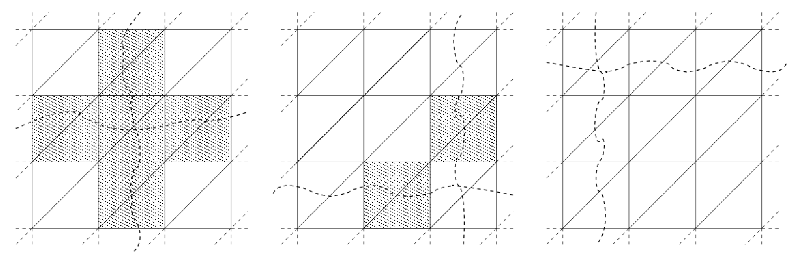
Figure 11 illustrates a section of a mesh whose nodes have been partitioned in three different ways. As outlined in the previous section, the parallel strategy is to lock elements cut by the graph partition while the remaining parts of the mesh in each domain are adapted. Clearly, this does not require interprocess communication.
Because halo elements were locked in place during the adaptive process there will in general exist elements, among and near previously locked elements, which are relatively suboptimal from an error control perspective. In addition, the mesh adaptivity will generally introduce a load-imbalance due to the addition and removal of mesh resolution. Both of these issues may be addressed simultaneously by repartitioning in such a way as to perturb the partition away from regions of the mesh which require further optimisation, while at the same time seeking to balance the final number of nodes per partition. This is accomplished through the application of suitable edge-weights and node-weights in the graph repartitioning calculation.
The graph partitioning problem involves the division of a graph, G = (V,E), into N partitions, G1,...,GN, such that there are approximately the same number of vertices, |V p|, per partition and the number of graph edges, |Ecut|, cut by the partitioning is minimised. For the work presented here, the publicly available graph partitioner ParMETIS 7 was used. This uses a fast k-way, multilevel based method which provides a selection of graph-partitioning strategies while allowing the application of weights on both the edges and vertices of the graph. The three principal parallel repartitioning methods relevant to the discussion here are scratch, scratch-remapping and diffusion methods (Schloegel et al., 1997). In the first approach, a new partitioning is calculated in parallel from scratch using multilevel graph partitioning methods. The resulting graph partition has little dependence on the initial graph partitioning. While this approach gives good quality load-balance and edge-cut it generally leads to significant data migration. Scratch-remapping curtails this problem by remapping the partitioning obtained from scratch onto the original, maximising overlap between partitions and thus minimising the data migration. The amount of data migration can be further reduced using the diffusion method, which takes an existing graph partition and only modifies it sufficiently to re-balance the partitioning. While this method is fast and results in the least data migration, the method tends to give a higher edge-cut. Indeed, it was observed that the partitions can become fragmented after repeated repartitioning using the diffusion method. The strategy is to apply diffusion by default to minimise data migration and to apply scratch-remap periodically to remove any islands that might occur. In this work a scratch-remap partitioning is always computed at the last adapt iteration because of the relatively low computational cost, and the importance of a good quality partitioning for the rest of the computation
A suitable perturbation of the graph partition is achieved through the application of edge weights to the graph when repartitioning. Simply applying high edge weights to regions which were previously locked (because of a graph partition) can encourage unnecessary mesh migration between processes as not all regions which were previously locked are in need of optimisation. The edge weights are derived by first defining the function Fl in terms of the worst of the elements sharing it:
 | (5) |
where Fe  > 0 is the element functional used by the serial mesh optimisation
algorithm (Pain et al., 2001). As high values of Fl identify regions of poor mesh
quality, high edge weight values are applied to discourage the graph partition from
cutting these edges. When the graph partitioning calculates the edge cut (one of the
metrics to be minimised by the graph partition) of a graph partition it sums
the edge weights rather than counting the number of edges cut by the
partition. Due to the nature of the Kernighan-Lin type refinement algorithm
(Kernighgan and Lin, 1970) used within ParMETIS and other k-way multilevel
graph-partitioners, (e.g. Hendrickson and Leland (1995); Karypis and
Kumar (1998); Walshaw et al. (1997)), edge weights are required to be
integer. For this reason Fl need to be remapped to Wl ℤ+, and must
be suitably distributed so as to ensure that poor elements are effectively
impenetrable by the new partitioning. In this work we define the mapping as:
> 0 is the element functional used by the serial mesh optimisation
algorithm (Pain et al., 2001). As high values of Fl identify regions of poor mesh
quality, high edge weight values are applied to discourage the graph partition from
cutting these edges. When the graph partitioning calculates the edge cut (one of the
metrics to be minimised by the graph partition) of a graph partition it sums
the edge weights rather than counting the number of edges cut by the
partition. Due to the nature of the Kernighan-Lin type refinement algorithm
(Kernighgan and Lin, 1970) used within ParMETIS and other k-way multilevel
graph-partitioners, (e.g. Hendrickson and Leland (1995); Karypis and
Kumar (1998); Walshaw et al. (1997)), edge weights are required to be
integer. For this reason Fl need to be remapped to Wl ℤ+, and must
be suitably distributed so as to ensure that poor elements are effectively
impenetrable by the new partitioning. In this work we define the mapping as:
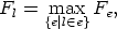
As mesh optimisation may be incomplete when the graph-partitioning is first performed it is important to be able to estimate the post-adaptation node density. The formulation of the mesh optimisation method makes it straightforward to estimate the local increase or decrease in element density. However, the predicted number of nodes after optimisation is not as readily available. This issue can be resolved by first realizing that what is important for load-balancing is the relative weight of nodes with respect to each other. Secondly, a linear relationship between the local number of elements and the number of nodes in the vicinity of a vertex can be assumed. The fractional increase in number of elements, αe, for a given element e, can be approximated by:
 |
where Ṽe is the volume of the element in metric space and γ is the volume of an
ideal element in metric space (i.e. the volume of a tetrahedron with unit edge
lengths). Assuming that the number of nodes varies linearly with the number of
elements in a mesh, the fractional increase in the number of nodes, ηn , can be
approximated by:
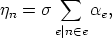 |
where σ is a proportionality constant, and n e states that node n is contained in
element e. As was the case with edge weights, ηn must be remapped to
wn ℤ+ ≥ 1, for example:
 |
where ∥ ∥∞ is the maximum value of ηn for all nodes. This nodal weighting is then
assigned to the computational mesh so that a graph partitioner can compute a
partition balancing the predicted number of nodes rather than the current number
of nodes per partition.
∥∞ is the maximum value of ηn for all nodes. This nodal weighting is then
assigned to the computational mesh so that a graph partitioner can compute a
partition balancing the predicted number of nodes rather than the current number
of nodes per partition.
After a new repartitioning is calculated, it is necessary to migrate appropriate
subsections between processes to achieve this repartitioning. Data migration (or
data remapping) is required to satisfy a graph repartitioning calculated in response
to a load-imbalance across processes. The graph repartitioning is expressed as a
redistribution of mesh nodes,  = (dn),n = 1,...,N, where dn = p specifies the new
process, p, that node n is assigned to.
= (dn),n = 1,...,N, where dn = p specifies the new
process, p, that node n is assigned to.
It is worth noting that the data structures associated with the mesh in mesh optimisation methods is in general much less complex than those associated with hierarchical based mesh refinement methods due to the fact that there is no mesh hierarchy (e.g. Ozturan (1995); Jimack (1998); Selwood and Berzins (1999)). This means that the cost of data remapping can potentially be much less than in hierarchical refinement methods.
Given the new graph partition,  , the first step is to determine the minimum set of
data that needs to be communicated in order to satisfy the new mapping. By doing
this, inter-process communication is minimised and there is no need to check for
the duplication of mesh objects. Each element, e, in a partition is considered in
turn. Two logical arrays,
, the first step is to determine the minimum set of
data that needs to be communicated in order to satisfy the new mapping. By doing
this, inter-process communication is minimised and there is no need to check for
the duplication of mesh objects. Each element, e, in a partition is considered in
turn. Two logical arrays,  and
and  , of length P (number of partitions) are defined
as:
, of length P (number of partitions) are defined
as:
To facilitate the discussion here, a node is said to be owned by a process if it is contained in the graph partition assigned to the process in question. The element is flagged if it is required on this process under the new partitioning (i.e. if Bp). Next, the owner of element e can be uniquely defined as the minimum-node-owner of e — that is to say the minimum rank of the owners on the nodes defining the element. If the current process is the owner of e, then e is listed to be sent to each process where (¬Ap) ∧Bp. Next the nodes on the element are checked. If element e has been flagged as a future element (i.e. an element required under the new partitioning) then each node in e is flagged as a future node, thus new halo nodes as well as new owned nodes are flagged to be kept. For a node in e to be listed to be sent to a process p it first must be owned by the current process and secondly (¬Ap) ∧ Bp must be true. It should be apparent that each node will be considered multiple times as it is referenced by different elements.
Define a mesh  which has been divided into P sub-domains such that
= 1 ∪2 ∪ ...P . In the context of repartitioning this can be rewritten as
= 1*∪
2*∪ ...
P * where
p* denotes the new sub-domain assigned to
process p. In both of these cases the sub-domain includes the nodes and elements in
the halo region. The notation p′ will be used to indicate the sub-domain p
excluding the halo elements and those nodes not owned by process p. In addition
p = l denotes the local process/domain. Using these definitions, the list of nodes
and elements a process must send to each other process can be determined using
Algorithm 1. At this point the minimum amount of information which must be sent
by each process to each other process, to satisfy the new graph-partitioning, has
been determined.
which has been divided into P sub-domains such that
= 1 ∪2 ∪ ...P . In the context of repartitioning this can be rewritten as
= 1*∪
2*∪ ...
P * where
p* denotes the new sub-domain assigned to
process p. In both of these cases the sub-domain includes the nodes and elements in
the halo region. The notation p′ will be used to indicate the sub-domain p
excluding the halo elements and those nodes not owned by process p. In addition
p = l denotes the local process/domain. Using these definitions, the list of nodes
and elements a process must send to each other process can be determined using
Algorithm 1. At this point the minimum amount of information which must be sent
by each process to each other process, to satisfy the new graph-partitioning, has
been determined.
|
Algorithm 1. find_entities_to_send(mesh)
Initialise nodes_to_process
Initialise elements_to_process for e = 1 to |elements| do {Create lists of nodes and elements to send to each process.} for p {p|e p*} do
if (n l′)&(n p*)&(n ⁄
p) then
nodes_to_processp ← n end if end for if (get_owner(e) ≡ pl)&(e Gp*)&(e ⁄ G
p) then
elements_to_processp ← e end if end for return nodes_to_process, elements_to_process |
After the information which is to be migrated has been identified, it is serialised (i.e. copied into a continuous buffer) and communicated. Node numbers must be specified in terms of their global node numbering rather than the node numbering local to a partition. An important outcome is that all data which needs to be migrated between two processes is performed in a single communication. The communication is efficiently implemented using non-blocking sends and receives with a preceding blocking probe, see Algorithm 2. Firstly, all the non-blocking sends are set up, including those whose message length is zero. Messages of zero length and the probe are unavoidable as a process has no prior knowledge of what information it should receive from other processes. Next the number of processes -1 is looped over, each time executing a blocking probe for a communication from any process (i.e. MPI_ANY_SOURCE). On a successful probe the sending process is identified and the size of the message being received from the process is read. If the message size is non-zero then a receive buffer is allocated and a non-blocking receive initialised. After all the receives have been set up, the algorithm waits for all non-blocking communications to complete.
|
Algorithm 2. AllSendRecv(packed_data)
for p = 1 to P do
MPI_ISend(data=packed_data_p, destination=p) end for for p = 1 to P do MPI_Probe(MPI_ANY _SOURCE,MPI_ANY _TAG) source ← find_source() data_size ← find_data_size() receive_buffersource ← allocate_receive_buffer(data_size) MPI_IRecv(data = receive_buffersource,source = source) end for MPI_Waitall() return |
After a process has received all its messages, it has enough data to construct its
new partition complete with its halo information. Using global node numbering, the
new halos are easily constructed without further communication. For each element
shared we loop though each node, n, in that element. If that node is owned
by the current process then every other node in the element owned by
process p, where p is not the current process, is inserted into the send list
for p,  p. On the other hand, if that node is owned by process p, where
p is not the current process, then it is inserted into the receive list for
p,
p. On the other hand, if that node is owned by process p, where
p is not the current process, then it is inserted into the receive list for
p,  p. The send and receive lists are then sorted using the global node
numbering resulting in the ith node being sent from process p to process q
referencing the same node as the ith node being received from process p by
q.
p. The send and receive lists are then sorted using the global node
numbering resulting in the ith node being sent from process p to process q
referencing the same node as the ith node being received from process p by
q.
After data migration, mesh adaptivity is reapplied if necessary. As suboptimal elements are only at or near previously locked elements, subsequent mesh adaptivity iterations are computationally inexpensive.
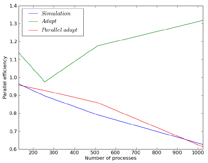
A scalability analysis of both the parallel mesh optimisation algorithm and of the complete CFD model was performed. This allows the performance of the parallel mesh optimisation method to be evaluated in the context of a ”real” application. In this work we focus on the strong scaling.
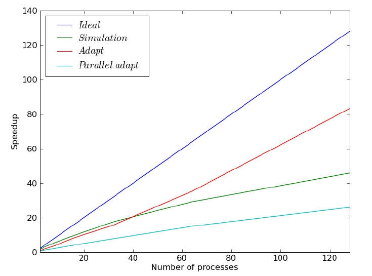
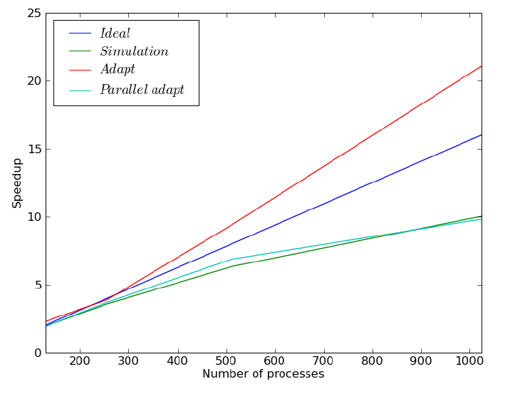
The differentially heated rotating annulus benchmark was used to evaluate the scalability of mesh adaptivity. A scalability analysis of both the parallel mesh optimisation algorithm and of the complete GFD model was performed. This allows the performance of the parallel mesh optimisation method to be evaluated in the context of a ”real” application. In this work we focused on the strong scaling. Two different problem sizes were considered for the experiments here: 0.1 million node mesh was run on 1, 2, 4, 8, 16, 32, 64 and 128 processors (see below left column); 2.0 million node mesh was run on 64, 128, 256, 512 and 1024 processors. In this experiment GMRES and EISENSTAT, implemented within PETSc, were used as the solver and pre- conditioner pair for momentum and temperature. Conjugate gradients and HYPRE’s BoomerAMG algebraic multigrid pre-conditioner were used when solving for pressure.
|
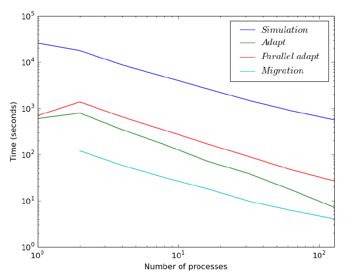
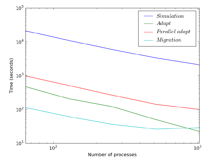
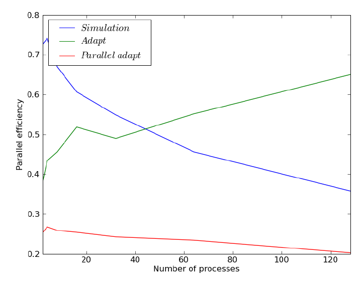
In figure 4.2, the absolute wall clock times of the simulation are plotted alongside mesh adaption on a log-log scale. In these experiments, mesh adaptivity represents approximately 5% of the total execution time. However, in general the proportion of the time spent adapting the mesh depends on many different factors; these include the nature of the problem being simulated and the frequency at which mesh adaptivity is applied. In all experiments a speedup is observed with an increase in number of processes. The parallel efficiency, E(N,P), for a problem of size N, running across P processes, is defined as:
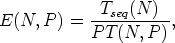 |
where T(N,P) is the runtime of the parallel algorithm, and Tseq(N) is the runtime of the sequential algorithm.
The drop in overall parallel efficiency for increasing number of processes is consistent with this being a fixed size problem where the computation/communication ratio decreases as the number of processes increases; this is seen as the relative difference between the mean number of owned nodes, and total number of nodes. For example, running the 100k node problem on 128 processes resulted in approximately 800 owned nodes per partition with approximately 700 halo nodes; running the 2m node problem on 1024 processes resulted in approximately 2000 owned nodes per partition with approximately 1400 halo nodes. By plotting separately the parallel efficiency of the pure adaptive part of the algorithm, along with the parallel efficiency of the parallel adaptive algorithm, it is clear that drop in efficiency is due the data migration/re-balancing overhead rather than imbalance in the serial mesh adaptivity operation. This application may be seen as a limiting case in that the work mesh adaptivity performed was approximately equidistributed throughout the domain, and therefore required the maximum amount of data migration.
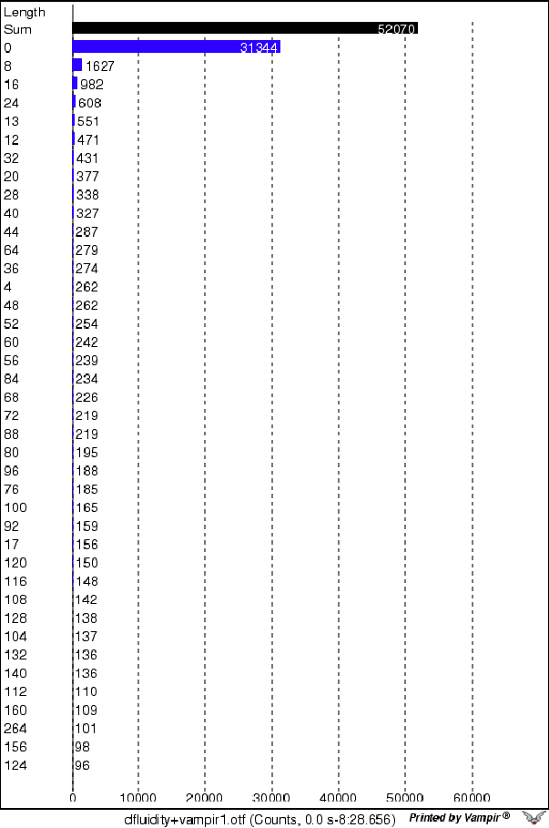
The fine grained profiling with Vampir has also been done within the adaptivity part. This revealed multiple redundant zero size message communications (using MPI_Isend and MPI_Ireceive) in ParMETIS (see Fig. 13). Since the cost of data migration in adaptivity is very low, it is not deserved to do further investigation at the moment.
Fluidity-ICOM output files containing simulation data are managed using the Visualization Toolkit (VTK - please refer to the website http://www.vtk.org/). VTK tools adopt the .vtu file format for unstructured grids: for each N dump times, the simulationname_N.vtu file is created, containing the output data of the simulation. This file contains a snapshot of the run at the time step immediately proceeding the dump time. For example, if the time step is set to three seconds, and the dump period to 10 seconds, the first dump will occur at 12 seconds.
When running a simulation in parallel, the data are stored both in both .vtu and .pvtu files. The .vtu files contain each of the output data for each partition of the parallelised mesh, with the file name simulationName_P_N.vtu where P is the processor number and N is the dump number. The .pvtu files contain the general output data for the whole mesh, again ordered by dump number.
The interleaved I/O is applied to vtu output. Suppose the total number of cores is N used in Fluidity-ICOM applications. Each process of a parallel application writes its data to several private files (mesh files, vtu file), This files-per-process pattern creates 5N (for a 3D mesh) for an application run of N processes. The performance of each processs file write is governed by serial I/O. However, this pattern constitutes the simplest implementation of parallel I/O, relying on some associated improvement in I/O performance from a parallel file system such as Lustre. However, at large process counts (large number of files) metadata operations may hinder overall performance. Additionally, at large process counts (large number of files) OSS and OST contention will hinder overall performance.
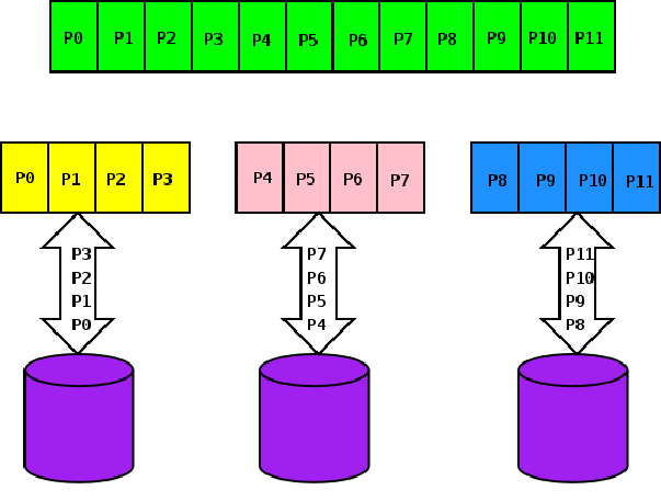
The interleaved I/O use a subset of application processes to perform I/O at the
I/O stage. This action will limit the number of requests hitting the metadata server
during I/O stage, thereby improving performance. Careful tuning of both the
number of writers and rank order can also give better performance. The total
writers is int( + 0.5). See Figure (14). Here, the total of 12 cores has been
divided into three groups, the processes in each group output their own files
following their rank order. At the end of the output operation processors wait for
all other processes to complete.
+ 0.5). See Figure (14). Here, the total of 12 cores has been
divided into three groups, the processes in each group output their own files
following their rank order. At the end of the output operation processors wait for
all other processes to complete.
A performance analysis has been undertaken with gyre test case (around 10 million mesh vertices). The conclusions are as follows:
This has been an ongoing process throughout the lifetime of the project. Several ’code sprints’ have been undertaken where large sections of the code was rewritten. Notably, one of the sprints generated a 200 page manual for the code.
From a starting point where the code was only routinely run on 64 cores on a local cluster, this Fluidity-ICOM dCSE project has significantly improved the performance of the code to enable efficient usage of large high performance computing systems such as the HECToR Cray XT4. Presently the code is now scaling well up to 4096 cores on HECToR. Runs on even larger core counts could be achieved if suitably partitioned datasets existed, these are currently under construction. The current barrier to running larger problem sizes is the memory footprint and computational cost of preprocessing tools - specifically the initial domain decomposition which is essentially a serial bottle neck.
Porting, developing and analysing the Fluidity-ICOM package revealed problems with the HECToR software development environment that were outside our control. Many have been resolved after a series of queries were raised with the NAG Support Team. However, several issues remain. In particular, the outstanding queries on PGI compilers not accepting standard Fortran constructs, and problems with CrayPAT profiling.
Python 2.6.* is tested and widely used within Fluidity-ICOM for the user interface, user-defined functions and for diagnostic tools and problem setup. The python interface removes the need for recompiling the code (which takes more than half hour) when input parameters change and problems are setup. It requires setup tools for Fluidity-ICOM builds, Python-4suite and Python-XML for options file parsing, and highly recommended extensions, such as scipy and numpy, for custom function use within Fluidity-ICOM. There were several Python modules missing on HECToR, several queries (Q44656, Q48686, Q51892, Q52507, Q64917 (submitted by Jon Hill from AMCG)) have been submitted, and Python-CNL module has been set up for all above queries by NAG support team.
Several PGI compilers bugs were triggered by Fluidity-ICOM. Testing from pgi/8.0.1 to pgi/9.0.4 has been made. New bugs and compiling faults came out with each round of testing. There have been bug reports raised for Fortran pointer dereference and Fortran generic interfaces, which are widely used in the code. Queries (Q43721, Q52502) have been submitted to the HECToR help desk. To date these issues have not been resolved and temporary workarounds in the Fortran source code have been applied.
Cotter, C., Ham, D., Pain, C., 2009. A mixed discontinuous/continuous finite element pair for shallow-water ocean modelling. Ocean Modelling 26, 86–90.
Ford, R., Pain, C., Piggott, M., Goddard, A., de Oliveira, C., Umpleby, A., 2004. A Nonhydrostatic Finite-Element Model for Three-Dimensional Stratified Oceanic Flows. Part I: Model Formulation. Monthly Weather Review 132 (12), 2816–2831.
Gorman, G., Pain, C., Piggott, M., Umpleby, A., Farrell, P., Maddison, J., 2009. Interleaved parallel tetrahedral mesh optimisation and dynamic load-balancing. Adaptive Modelling and Simulation 2009, 101–104.
Gorman, G., Piggott, M., Wells, M., et al, 2008. A systematic approach to unstructured mesh generation for ocean modelling using GMT and Terreno. Computers & Geosciences 34, 1721–1731.
Gorman, G. J., Piggott, M. D., Pain, C. C., de Oliveira, C. R. E., Umpleby, A. P., Goddard, A. J. H., 2006. Optimisation based bathymetry approximation through constrained unstructured mesh adaptivity. Ocean Modelling 12(3-4), 436–452.
Gresho, P., Sani, R., 1998. Incompressible Flow and the Finite Element Method.
Hendrickson, B., Leland, R., 1995. A multilevel algorithm for partitioning graphs. In: Proc. Supercomputing ’95. Formerly, Technical Report SAND93-1301 (1993).
Jimack, P. K., 1998. Techniques for parallel adaptivity. In: Topping, B. H. V. (Ed.), Parallel and Distributed Processing for Computational Mechanics II. Saxe-Coburg Publications.
Karypis, G., Kumar, V., 1998. A fast and high quality multilevel scheme for partitioning irregular graphs. SIAM Journal on Scientific Computing 20 (1), 359–392.
Kernighgan, B. W., Lin, S., 1970. An efficient procedure for partitioning graphs. Bell Systems Technical Journal 49.
Kramer, S., Cotter, C., Pain, C., 2010. Solving the Poisson equation on small aspect ratio domains using unstructured meshes. Ocean Modelling, submitted, arXiv:0912.2194.
Kramer, S., Pain, C., 2010. Modelling the free surface using fully unstructured meshes. In preparation.
Ozturan, C., 1995. Distributed environment and load balancing for adaptive unstructured meshes. Ph.D. thesis, Rensselaer Polytechnic Institute, Troy, New York.
Pain, C., Piggott, M., et al., 2005. Three-dimensional unstructured mesh ocean modelling. Ocean Modelling 10, 5–33.
Pain, C., Umpleby, A., de Oliveira, C., Goddard, A., 2001. Tetrahedral mesh optimisation and adaptivity for steady-state and transient finite element calculations. Computational Methods in Applied Mechanics and Engineering 190, 3771–3796.
Schloegel, K., Karypis, G., Kumar, V., 1997. Multilevel diffusion schemes for repartitioning of adaptive meshes. Journal of Parallel and Distributed Computing 47 (2), 109–124.
Selwood, P. M., Berzins, M., 1999. Parallel unstructured tetrahedral mesh adaptation: algorithms, implementation and scalability. Concurrency: Practice and Experience 11 (14), 863–884.
Walshaw, C., Cross, M., Everett, M., 1997. Parallel dynamic graph partitioning for adaptive unstructured meshes. Journal of Parallel and distributed Computing 47, 102–108.