EPCC, The University of Edinburgh,
James Clerk Maxwell Building,
Mayfield Road,
Edinburgh,
EH9 3JZ, UK
8th June 2010
Abstract
This report presents the results of a dCSE project to improve the scalability of turbulence applications (principally EBL) from what is currently hundreds of cores to thousands of cores. This is necessary in order to exploit HECToR properly and to allow advances in the scientific investigations that use these applications. An existing code has been re-engineered. For a problem size that previously would have used a maximum of 365 cores, very good scaling has been demonstrated up to 11,000 cores and good scaling up to 14,000 cores. Furthermore, because of memory limitations, this size of problem was beyond the scope of the original code. These improvements in scalability have been achieved by implementing a two-dimensional domain decomposition (a.k.a. pencil decomposition).
This is the final report for a dCSE project that ran from 1st April 2009 to 31st March 2010.
Spectral codes that perform a one dimensional decomposition of problems set in three spatial dimensions do not scale well on today’s large computers which contain thousands of cores. This is because they are limited in the number of cores they can exploit by the the smallest of the number of collocation points (or some factor in the order of one thereof) taken over the three dimensions. Even when using the maximum number of cores allowed by the decomposition for a given size of problem domain, the load on a core (in terms of both the amount of computation and storage required) increases with something like the square of the a typical linear dimension characterizing the size of the problem.
By employing a two dimensional decomposition the limit on the number of cores that can be used can be raised and the growth in the load on a core can be reduced to something like a linear dependence on a typical dimension describing the problem. This happy state of affairs is, of course, limited by the maximum number of cores that are available to a job and by the increasing need to move data between cores.
The goal of this project was to demonstrate that, by employing two dimensional decompositions of the problem domain and despite the increased communication overhead, three dimensional spectral codes can be made to scale from the current hundreds of cores to thousands of cores. The spectral codes to be considered were EBL, SWT and SS3F. EBL was to be tackled first with SWT and SS3F being considered as time allowed. In the event SWT and SS3F have not been tackled as EBL took up all of the alloted time, however the results for EBL are very good and suggest that SWT and SS3F would benefit from a similar treatment.
The work reported here differs from previous work in a number of respects:
EBL (named after the Ekman Boundary Layer) is used to investigate pressure driven flow over a single surface, located in the x-z plane. For this problem trigonometric functions form a good spectral basis with respect to the x and z direction which have periodic boundary conditions imposed on them. The y direction is normal to the fixed surface and Jacobi polynomials offer a good spectral basis with respect to the boundary conditions imposed in that direction. The application calculates the forcing terms in position space and performs the Runge-Kutta steps for the time evolution in the spectral space. As a consequence frequent transformations between position space and spectral space are required. EBL and results obtained using it are discussed in [Coleman et al. 1999, Spalart et al. 2008, Spalart et al. 2009]
The first version of the code was written in the mid 1980s at NASA Ames Research Center by Dr Philippe Spalart, using the algorithm described in [Spalart et al. 1991]. Development and maintenance by Dr Gary Coleman followed in the 1990s. In 2002-2003, it was converted from Vectoral to Fortran, and parallelised using MPI, by Drs Mike Ashworth and Roderick Johnstone of Daresbury Laboratory, in support of the UK Turbulence Consortium. This code was used on HPCx, and relies on either the IBM ESSL or the FFTW3 libraries to perform Fourier transforms. It also requires BLAS and LAPACK.
The Reynolds number of a flow determines the size of the smallest domain that may be used to study it. This means that when the EBL3 code is run there is a minimum size of lattice that may be used and that the lattice whilst cuboidal is not a cube.
This dCSE project was carried out on HECToR, the UK National Supercomputing service. Full details of the system are available here.
The work reported here was carried out whilst HECToR was in its ’Phase 2a’ configuration which includes a scalar MPP XT4 system, a vector system, and storage systems. The XT4 comprises 1416 compute blades, each of which has 4 quad-core processor sockets. Each quad-core socket shares 8 GB of memory. In addition there are 24 service blades, each with 2 dual-core processor sockets. They act as login nodes and controllers for I/O and for the network. The vector system includes 28 vector compute nodes.
The results were obtained by running EBL on the XT4. The vector system was not used.
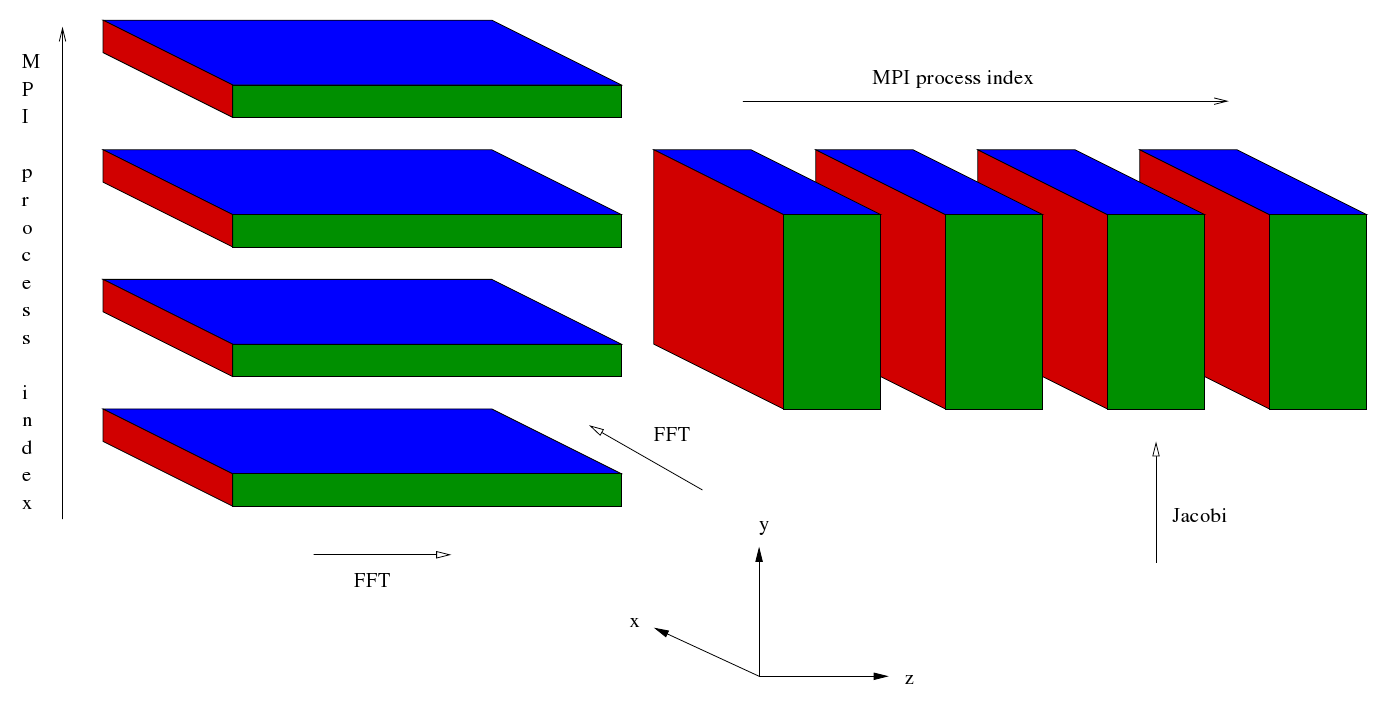
To perform a spectral transformation of all three dimensions a sequence of one dimensional transforms is performed. For each of these one dimensional transformatations EBL3 uses a ‘plane’ (a.k.a. ‘slice’ or ‘slab’) decomposition of the domain. That is one of the dimensions, Y say, is divided up as evenly as possible for distribution across the allocated number of cores. For each Y index allocated to a given core1 all of the indices in the remaining two dimensions, Z and X in this case, are allocated to that same core. On each core a loop over the allocated Y values is performed. Inside the loop a transform is performed on one of the other dimensions, Z say. Once the loop is completed the data is transposed so that it is easy to transform the second complete dimension, X in this case. This transpose is local to the core.
Currently results are slowly being generated for Re = 2828 on a 1344 × 273 × 4032 (Nx × Ny × Nz) lattice, but this version of the code has reached the end of its life as, whilst it can be run on HECToR, it cannot be used to study higher Reynolds numbers than those already studied because of the limitations on the memory available to it and the time it would take to run.
A brief description of the working of this code follows. This description focuses on the movement of data between processors and on the spectral transformations that occur.
After some initialisation the master processor reads in some data and broadcasts it to the rest of the processors. Then the following sequence is executed beginning at Step 6b.
The Fourier transforms in Step 3b and Step 3d are inside a loop which runs from 1 to 6 whilst the Fourier transforms in Step 3e and Step 3g are inside a loop which runs from 4 to 6. This is mentioned here as it is no longer the case in the new code described below.
Figure 1
A short description of the new version of the EBL code follows. The description focuses on the movement of data between MPI processes (which correspond to cores) and on the spectral transformations that occur.
After some initialisation the master process reads in some data and broadcasts it to the rest of the MPI processes. Then a cartesian communicator, cart_comm, is created corresponding to a two dimensional grid of processes. Sub-communicators corresponding to the two dimensions are created - comm1 and comm2 respectively. The simulation starts off in entirely in wave space. Data for different values of Z are distributed along the first dimension of the process grid whilst data for different values of X are distributed along the second dimension of the process grid. For given values of Z and X the data corresponding to all values of Y are held (concentrated) in a single MPI process.
Four sets of Fourier transformations are planned. These are similar to the plans generated in the current EBL3 code but the number of transforms that are carried out by the plans is different. This is because in the case of a Fourier transform of the Z direction the X direction has been distributed across the second dimension of the process grid whilst in the case of a Fourier transform of the X direction the Z direction has been distributed across the second dimension of the process grid. Furthermore, the loops enclosing the FFTs mentioned at the end of the preceding section have been incorporated into the plans. After the FFTs have been planned the following sequence begins at Step 7b.
Note that
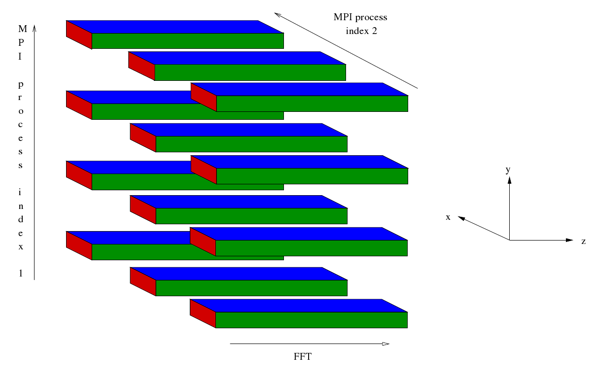
Figure 2
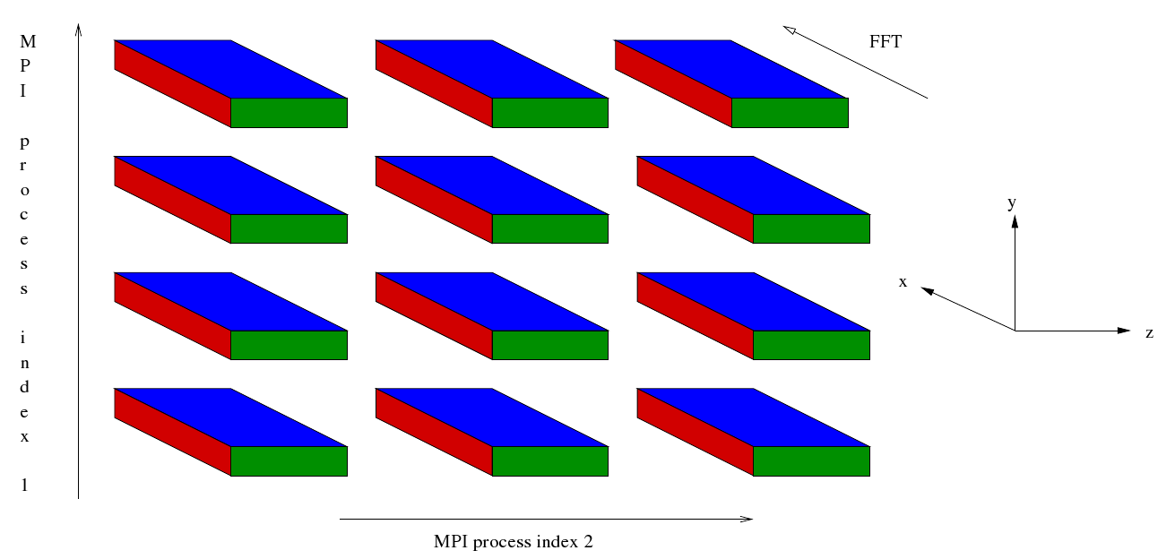
Figure 3
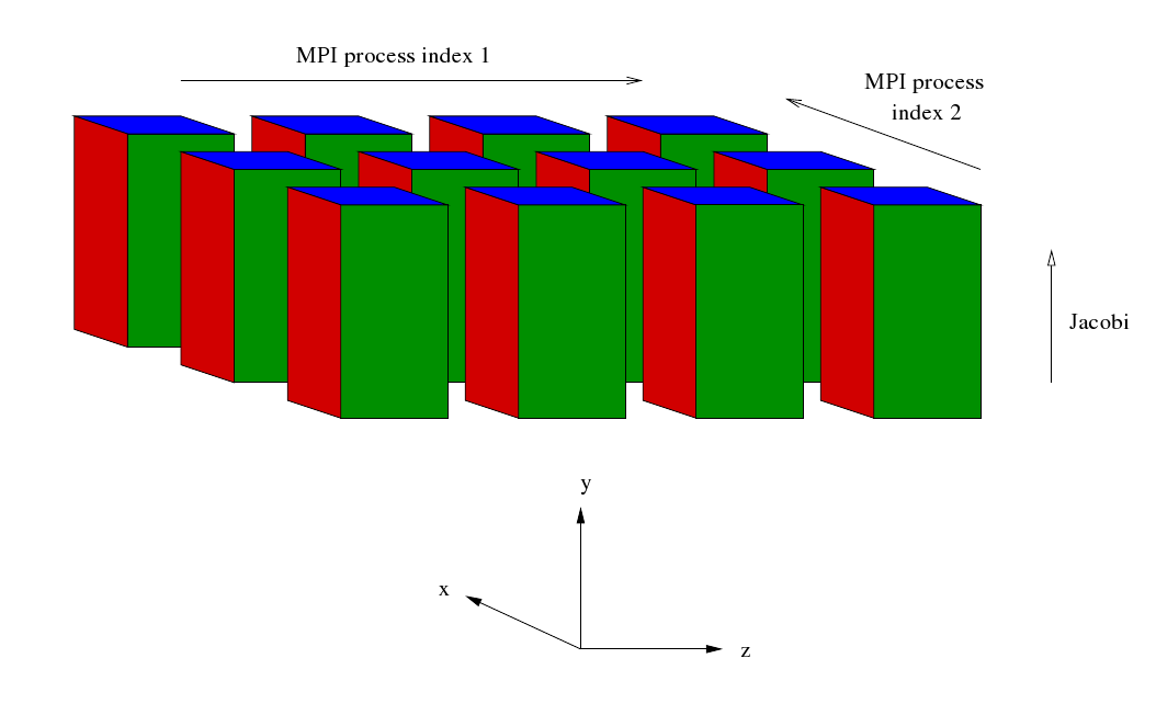
Figure 4
The Fortran compiler used was pgi 9.0.4. It was used with the flag -O3. The flag -fast was tried but dropped as the program did not work correctly when compiled with this flag.
Plans were generated by FFTW3 with the MEASURE algorithm. PATIENT and EXHAUSTIVE were tried but dropped because of the length of time they took to produce plans for large domain sizes. All three planning algorithms (MEASURE, PATIENT and EXHAUSTIVE) were tried out on one of the smaller domains. Using PATIENT and EXHAUSTIVE did not produce a significant increase in performance over using MEASURE. Only those results produced using MEASURE are reported below.
The new code distributes the computation across an nproc1 × nproc2 grid of MPI processes. If nproc2 is set to 1 the code behaves in a similar fashion to the current EBL3 code. The new code does not treat nproc=1 in any special way: it still makes its usual MPI calls even if they are unnecessary.
Because of the amount of memory available at each node the largest domain that can be studied with the current EBL code whilst employing all of the cores on a node is 1344 × 273 × 4032. The second largest size of interest that can be studied with the current code is 768 × 204 × 2304. For these domain sizes the performance of the current code was compared with that of the new code. Two measures were used in in the comparison: the average time for one of 30 Runge-Kutta steps and the minimum time for the same 30 Runge-Kutta steps. The results were as follows.
| cores = 204 | Original | New | Change |
| Average | 3.10 � 0.04 | 3.14 � 0.04 | 1% |
| Minimum | 2.84 | 2.97 | 5% |
| cores = 273 | Original | New | Change |
| Average | 9.89 � 0.16 | 10.24 � 0.14 | 4% |
| Minimum | 8.97 | 9.61 | 7% |
In these cases the performance of the new code is worse than that of the current code and the difference is greater for the larger domain size, however the effect is not great and as we shall see it does not prevent either an improvement in performance for currently tractable domain sizes (by employing more cores) or the investigation of larger domain sizes.
The scaling behaviour of the new code has been investigated for Re = 4000 (Nx× Ny × Nz = 2432 × 365 × 7232). The largest number of cores that the current code could (in principle) exploit is 365, however this cannot be done in practice on HECToR because of the length of time the code would take to execute and the memory that would be required per core. In order, therefore, to provide a standard against which the performance of the code may be measured the performance for the new code running on a 365 × 8 grid of MPI processes has been extrapolated according to perfect scaling.
The principal investigation involved keeping the size of the first dimension of the MPI process grid fixed at 365 and increasing the size of the second dimension. The values of this second dimension for which results were obtained are: 8, 16, 24, 32, 40 and 44. The number of cores employed by the code were: 2920, 5840, 8760, 11680, 14600 and 16060 respectively, the last being the largest number of cores that could be used in this progression. Two measures of performance were used: the maximum number of Runge-Kutta steps per minute and the average number of Runge-Kutta steps per minute. Qualitatively the results are very similar.
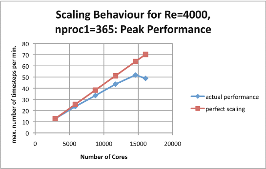
Figure 5
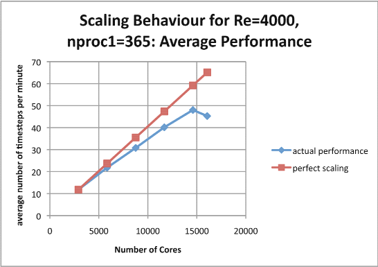
Figure 6
Scaling factors can be calculated from both sets of measurements and agree to two significant figures (except for when the number of cores is 16,060 when the two methods give 0.69 and 0.70 respectively). Here are the figures:
| Cores | Scaling Factor |
| 2,920 | 1 |
| 5,840 | 0.92 |
| 8,760 | 0.87 |
| 11,680 | 0.85 |
| 14,600 | 0.81 |
| 16,060 | 0.69 |
Examination of these graphs shows that the code scales very well up to 11,000 cores and the scaling is still good at 14,000 cores. After that, however the performance degrades and for 16,000 cores the performance is worse than that for 14,000 cores. Presumably this is because of the increased cost of the communications between the MPI processes.
The next value of physical interest is Re = 5656 (which corresponds to Nx× Ny × Nz = 468 × 515 × 14400). This could, perhaps, have been run on HECToR on a 515 × 31 (= 15,965) process grid but this has not been attempted.
For Re = 4000 an MPI process grid with nproc1 ≠ 365 was tried to see how it affected the performance of the code. The results given below were obtained using an executable instrumented with CrayPat and each has been calculated from 183 values. For each process grid the average time for a Runge-Kutta step has been given as well as the minimum time.
| Grid | Average | Minimum |
| 365 × 24 | 1.90 s | 1.76 s |
| 73 × 120 | 2.52 s | 2.26 s |
It can be concluded that the change in geometry has degraded performance. The reason for this is discussed below.
In production runs the code will be run for tens of thousands of time steps so the time required to initiate a run is of little interest, and this is also the case for finalisation. For each process grid two runs were performed with different numbers of simulation steps (3 and 63 to be precise) in order to be able to subtract the effect of initialisation and finalisation. For 60 time steps in the middle of a run the following results were obtained from CrayPat.
| Grid | MPI | Etc | User | Total |
| 365 × 24 | 7327 | 6567 | 5711 | 19605 |
| 73 × 120 | 11664 | 7690 | 5561 | 24915 |
| Grid | MPI | Etc | User |
| 365 × 24 | 37% | 33% | 29% |
| 73 × 120 | 47% | 31% | 22% |
The amount (and proportion) of time spent in MPI calls is increased by the change in geometry. The reason for this can be seen by examining Step 4 of the algorithm set out in Section 3: the loop over Y values has only one iteration for the first grid but has five for the second grid, and this loop contains two ALLTOALLVs.
In the case of EBL, a 3 dimensional spectral code, it has been shown that the introduction of a two dimensional decomposition has enabled good scaling of the code to be extended from a few hundred cores to a many thousands of cores. A result of this is that the study of a higher Reynolds number has become practicable. There are other codes, SWT and SS3F, that could well benefit from a similar treatment but time did not allow this to be investigated.
The new version of the code has been run on HECToR XT6 during its early access period when it was located in the USA and there are plans to use it in further studies of the Ekman boundary layer. Now that this system has been transported to the UK the code has been installed on the new Phase 2b HECToR system and is available as the module “ebl”.
I would like to thank Dr. Roderick Johnstone and Dr. Gary Coleman for the support that they gave to me whilst I was carry out this work. Without the support of Roderick Johnstone in particular this work would have been impossible.
[Spalart et al. 1991] Spalart, P.R., Moser, R.D., and Rogers, M.M. (1991) "Spectral methods for the Navier-Stokes equations with one infinite and two periodic directions", JCP, 96, 297-324
[Coleman et al. 1999] Coleman, G.N. (1999) "Similarity Statistics from a Direct Numerical Simulation of the Neutrally Stratified Planetary Boundary Layer", J. Atmos. Sci. 56, 891
[Spalart et al. 2008] Spalart, P.R., Coleman, G.N., and Johnstone, R. (2008) "Direct numerical simulation of the Ekman layer: A step in Reynolds number, and cautious support for a log law with a shifted origin", Phys. Fluids 20, 101507
[Spalart et al. 2009] Spalart, P.R., Coleman, G.N., and Johnstone, R. (2009) "Retraction: “Direct numerical simulation of the Ekman layer: A step in Reynolds number, and cautious support for a log law with a shifted origin” [ Phys. Fluids 20, 101507 (2008) ]", Phys. Fluids 21, 109901 (2009)