This report documents the work performed during the dCSE
project titled “OPTIMISING THE PARALLELISATION OF A HARMONIC BALANCE
NAVIER-STOKES SOLVER FOR THE ULTRA-RAPID ANALYSIS OF WIND TURBINE,
TURBOMACHINERY AND AIRCRAFT WING PERIODIC FLOWS”. The project, undertaken at EPCC, The
University of Edinburgh, in conjunction with Dr M. Sergio Campobasso from the
Systems, Power and Energy Research Division of Glasgow University, aimed to
improve the overall performance of the COSA simulation code, thereby reducing
the computational resources required to undertake scientific simulations,
enabling more efficient use of the resources provided by the HECToR service
(and other HPC systems), and reducing the runtime required to undertake
simulations for large scale problems.
COSA is a novel CFD system based on the compressible
Navier-Stokes (NS) model for unsteady aerodynamics and aeroelasticity of fixed
structures, rotary wings and turbomachinery blades. The COSA code is written in
FORTRAN, and it includes a steady, a time domain (TD) [1-3] and a harmonic
balance (HB) [2] flow solver. All three solvers use a finite volume scheme with
structured multi-block grids. The integration of the steady and HB equations is
based on an explicit multigrid algorithm using a multi-stage Runge-Kutta (RK)
smoother. Solution of unsteady problems in the TD is obtained by using
Jameson’s dual-time stepping. Turbulent flow effects are modelled by means of
the two-equation K-ω Shear Stress Transport (SST) turbulence model of
Menter [1].
The COSA suite also uses Low-Speed Preconditioning [2,3],
which enables its use also for low-speed flows, such as those associated with horizontal
axis wind turbines (HAWT’s). All 3 COSA
solvers (steady, TD, and HB) have been parallelised, since their execution
requires large amounts of computational resources. There are three different parallelisations of
the current code[5,6]:
- OpenMP
- MPI
- Hybrid (mixed OpenMP and
MPI)
The OpenMP parallelisation can work for all three solvers,
with different parallelisations available over the blocks in the multi-block
grids, over the harmonics for the HB solver, and over the grid points for those
problems that use low numbers of blocks or harmonics (for instance a single
block, TD, simulation).
The MPI parallelisation distributes the blocks of the
multi-block grid over the available MPI processes to distribute the work of the
simulation. Communication is required between the blocks where data on the edge of blocks (called cuts in
COSA) needs to be communicated to neighbouring blocks (halo communications). The maximum number of processes that the MPI
parallelisation can use is limited by the number of geometric partitions (grid blocks) in the simulation.
The hybrid
parallelisation combines the MPI code with either the harmonic OpenMP
parallelisation or the grid point OpenMP parallelisation, depending on the
simulation being performed.
HECToR, a Cray XE6
computer, is the UK National Supercomputing Service. This project utilised the Phase 3 incarnation
of the system. Phase 3 of HECToR
consists of 2816 nodes, each containing two 16-core 2.3 GHz ’Interlagos’ AMD
Opteron processors per node, giving a total of 32 cores per node, with 1 GB of
memory per core. This configuration provides a machine with 90,112 cores in
total, 90TB of main memory, and a peak performance of over 800 TFlop/s.
Three different
test cases have been used for understanding the performance and runtime
characteristics of COSA, the details of these are provided next.
This test case is a HB analysis of a heaving and pitching
wing designed to extract energy from an oncoming air stream. The 512-block grid
has 262,144 cells, and 31 real harmonics are used. This HB analysis has the
same memory requirements of a steady flow analysis with more than 8 million
cells. Further details on the
aerodynamics of this device and the analysis of its efficiency based on COSA
time-domain simulations are reported in the articles [1,3].
The test case is that associated with the HB flow analysis
of the blade section at 90% span of a multi-megawatt horizontal axis wind
turbine operating in yawed wind. The analysis has been performed using both a
coarse and a fine grid, both consisting of 32 grid blocks. The coarse grid has
73728 cells, whereas the fine grid has 654336 cells. Further details on the
time-domain and HB COSA analyses of this problem are reported in the article
[2].
Test case 3 is a finer grid version of test case 2. In TC3,
the computational grid has 2048 blocks, and the grid has 4,194,304 cells. In
the simulations we have used 17 real harmonics.
Whilst the different parallelisations of COSA enable large simulations to be
performed correctly, and in a much shorter time than the serial code, the
efficiency of the different parallel implementations is not optimal. The OpenMP parallelisation allows simulations
to be run on local computers such as desktop machines, and small shared-memory
clusters, however it cannot be used on large scale resources. Furthermore, the OpenMP parallelisation did not
scale well even on small numbers of cores.
The MPI code is generally efficient, although there are some areas that
can be improved, but can only utilise a maximum number of cores equal to the
maximum number of grid blocks in the simulation. The hybrid code was developed to address this
restriction, enabling parallelisation that use more cores than the number of
blocks in the simulation, however it was less efficient than the pure MPI
parallelisation as it used the inefficient OpenMP functionality as well as the
reasonably efficient MPI functionality.
Therefore, this dCSE project aimed to improve COSA in the following two
areas to enable it to efficiently be used on HECToR:
1. Optimise MPI communications of the COSA HB
solver
2. Optimise the OpenMP and hybrid
parallelisation of the COSA HB solver
For the remainder of this report we will outline the current
performance of the existing COSA parallelisation in Section 2, discuss the
optimisation performed on the MPI code in Section 3, outline the initial
optimisation work undertaken on the hybrid code in Section 4, and further
advanced hybrid optimisation undertaken in Section 5. We will finish with summary of the work
undertaken and the overall performance benefits in the final section, Section
6.
The efficiency of the existing harmonic OpenMP parallelisation
has been assessed using test case 1. Figure
1 shows the runtime of the OpenMP parallelisation on a 32-core node of HECToR,
and it highlights a poor performance of the OpenMP parallelisation.
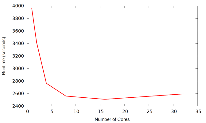
Figure 1:Runtime for the OpenMP code
for test case 1
The speedup of the MPI parallelisation of the code on the
same test case as the one used for the OpenMP parallel scaling study is shown
in Figure 2. The MPI code has much better scaling than the equivalent OpenMP functionality,
but it is still not optimal, particularly at larger process counts. The MPI code was designed to provide a
one-to-one correspondence to the functionality of the serial code and it sends
the dataset of one halo cell at a time rather than the dataset of all halo
cells associated with a particular grid cut (boundary between adjacent blocks)
at once. Although important in establishing correctness and confidence in the
parallelisation, this simplistic approach is inefficient. In an efficiently
implemented MPI code, increasing the size of the grid blocks without altering
the overall number of blocks should have a negligible impact on the MPI
efficiency, because the overall number of MPI communications does not vary
significantly, and the ratio between the time spent for actual computing and
communications remains about constant (this is because both the size of the MPI
messages and the number of operations of each block increases).
Conversely, in the MPI code, increasing the size of each
block reduces the MPI efficiency, because this operation results in a larger
number of small MPI messages. However,
in the code with an ideal parallelisation there would be a constant number of
messages, the size of which depends on the block size, rather than an increase
in the number of messages sent. An example is provided by the table below,
which reports the results of a scaling test of the existing MPI COSA HB solver
on HECToR Phase 2b. Test case 2 was used
for these benchmarking runs. As
expected, the MPI efficiency is higher for the coarse grid, as a consequence of
the substantially larger number of (small) MPI messages present in the fine
grid case.
|
Cores
|
1
|
2
|
4
|
8
|
16
|
32
|
|
Coarse grid speed-up
|
1.00
|
1.82
|
3.21
|
5.56
|
11.30
|
21.01
|
|
Fine grid speed-up
|
1.00
|
1.80
|
2.96
|
4.55
|
9.34
|
17.47
|
Table 1: Scaling of the original MPI
code using test case 2 with different mesh sizes
Aside from this issue, the existing MPI HB code has an
acceptable performance, also for larger problems, as demonstrated in Figure 2, where the speed-up of the
MPI code is plotted against the number of processes used.
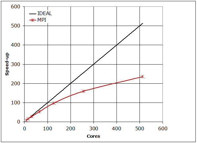
Figure 2: Parallel speedup of MPI code for test case 1
We also looked in detail at the performance of the MPI code,
profiling it with the Craypat performance analysis tool available on
HECToR. We obtained the following
profiling data using 512 MPI processes on test case 1.
Samp% | Samp
| Imb. |
Imb. |Group
|
| Samp | Samp%
| Function
|
| | |
PE=HIDE
100.0% | 63045.9 | -- |
-- |Total
|------------------------------------------------
| 78.8% |
49694.5 | -- | -- |USER
||-----------------------------------------------
|| 17.3% | 10911.0 | 596.0 |
5.2% |blsp_
|| 14.9% |
9415.1 | 630.9 | 6.3% |proflux_b_
|| 6.6% |
4143.6 | 393.4 | 8.7% |vflux_b_
|| 4.7% |
2933.7 | 739.3 | 20.1% |src_bhb_
|| 4.1% |
2554.6 | 289.4 | 10.2% |tridi_
|| 2.7% |
1709.7 | 368.3 | 17.7% |muscl_bi_
|| 2.7% |
1698.2 | 183.8 | 9.8% |cirs_b_
|| 2.7% |
1686.2 | 155.8 | 8.5% |bresid_
|| 2.6% |
1660.3 | 213.7 | 11.4% |muscl_bj_
|| 1.6% |
1020.4 | 128.6 | 11.2% |eig_ns_p_
|| 1.6% |
1011.3 | 190.7 | 15.9% |prec_bres_
|| 1.5% |
936.2 | 198.8 | 17.5% |lm_bviscoff_
|| 1.5% |
922.2 | 179.8 | 16.3% |bq_der_i_
|| 1.2% |
785.1 | 103.9 | 11.7% |bdeltat_
|| 1.2% |
782.9 | 210.1 | 21.2% |bq_der_j_
|| 1.2% |
727.7 | 101.3 | 12.2% |limit_j_
|| 1.1% |
708.3 | 212.7 | 23.1% |limit_i_
|| 1.1% |
698.0 | 124.0 | 15.1% |b_rtst_
|| 1.0% |
633.1 | 107.9 | 14.6% |cut_q_
||===============================================
| 14.7% |
9292.6 | -- | -- |MPI
||-----------------------------------------------
|| 10.2% |
6412.1 | 3715.9 | 36.7%
|MPI_WAITANY
|| 2.7% |
1704.2 | 170.8 | 9.1% |MPI_ISEND
||===============================================
| 6.4% |
4058.8 | -- | -- |ETC
||-----------------------------------------------
|| 1.4% |
886.5 | 127.5 | 12.6% |__c_mzero8
|| 1.2% |
731.8 | 251.2 | 25.6% |_int_malloc
|================================================
We can see that the majority of the runtime of COSA (around
80%) for this testcase is spent in user routines (i.e. the subroutines in the
COSA project), with around 15% of the runtime in MPI communications. Furthermore, we can see that there are 10
subroutines that take up around 60% of the overall runtime of the code. Therefore, we can identify those routines
that are critical for optimising the OpenMP performance (and therefore ensuring
that the hybrid code has good performance), and also which parts of the
communication functionality are dominating the MPI performance enabling us to
effectively target our work on the MPI optimisation. It should be noted that the above profiling
data was collected with the I/O in COSA turned off, so I/O costs have not been
profiled.
The primary focus for this work was to optimise the inefficient
MPI communications in COSA. The existing
code utilises non-blocking MPI communications, but for a large simulation there
can be as many as 5,000 messages sent between communicating processes at each Runge-Kutta
step. Optimising this was one of the
first steps in the dCSE. However, there
were a number of other areas that were also identified for optimisation in this
work. A number of places in the COSA
code use hand coded linear algebra functionality, it was decided to replace
this with the same functionality implemented in a linear algebra library. Furthermore, for large simulations the I/O
was seen to take up a large portion of the runtime so we also looked at
optimising that. The following
subsections will go into these optimisations in more detail.
As mentioned in the introduction to this section the current
MPI parallelisation can require a large number of messages to be send and
received to communicate “halo” or cut data to neighbouring processes. This is because the existing code sends small
parts of the boundary data to neighbouring processes at a time, with an example
of this shown in the following pseudo code:
do i = 0,boundary length
if(myblock1 .and. myblock2) then
do n = 0, 2*nharms
do ipde = 1, npde
copy 1st part of q2 to q1
copy 2nd part of q2 to q1
end do
end do
else if(myblock1) then
receive 1st part of q1
from remote process
receive 2nd part of q1
from remote process
else if(myblock2) then
send 1st part of q2 to remote process
send 2nd part of q2 to remote process
end if
end
do
Note that in the above pseudo code we can see that the MPI
communications have already been partially optimised, as they don’t send a
message for each element of the n
and ipde loops, they aggregate
the data to be sent or received into an array and then send that array, as
shown in the following code (which implements one of the send steps in the pseudo code above):
datasize = npde*((2*nharms)+1)
tempindex = 1
do n = 0, 2*nharms
do ipde = 1, npde
sendarray(tempindex,localsendnum) =
& q2(in1,jn1,ipde,n)
tempindex = tempindex + 1
end
do
end do
call sendblockdata(sendarray(1,localsendnum),iblk1,
& iblk2,datasize,sendrequests(localsendnum))
However, as the send and receive functionality is within a
loop, and for that loop the send and receive processes do not change (the same sender
and receiver are involved in all the communications for a given invocation of
the loop) it is possible to reduce all these send and receives down to one send
and one receive by further aggregating the data into a single send array and
using a single receive array.
We implemented such a scheme, which aggregated together
communications, at the expense of extra data storage (required to store the
aggregated data), and tested it with test case 1. All the communication functionality is
contained in routines named cutman_
in COSA. The results for HECToR are shown in Figure 3.
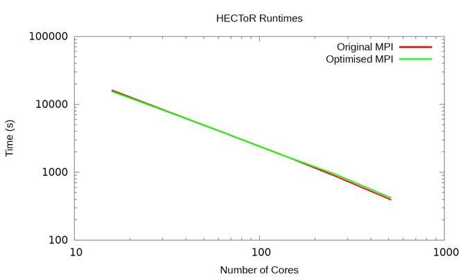
Figure 3: Runtime for the new MPI code vs the old MPI
code on HECToR using test case 1
We can see from Figure 3 that the optimised MPI
communication strategy has not improved the performance of the code; indeed the
original MPI code is slightly faster at 256 and 512 cores whereas the new MPI
code is slight faster at lower core counts.
This is contrary to what we expected so we investigate what was happening
in the code in more detail using the Scalasca[4] profiling tool.
We ran performance profiling using the test data outlined in
the previous Figures and discovered that the new MPI code does indeed
dramatically reduce the number of MPI messages sent by the cutman_ routines. Figure 4 and 5 show examples of the output of
the Scalasca tool showing message counts and data transfer sizes for the old
and new codes.
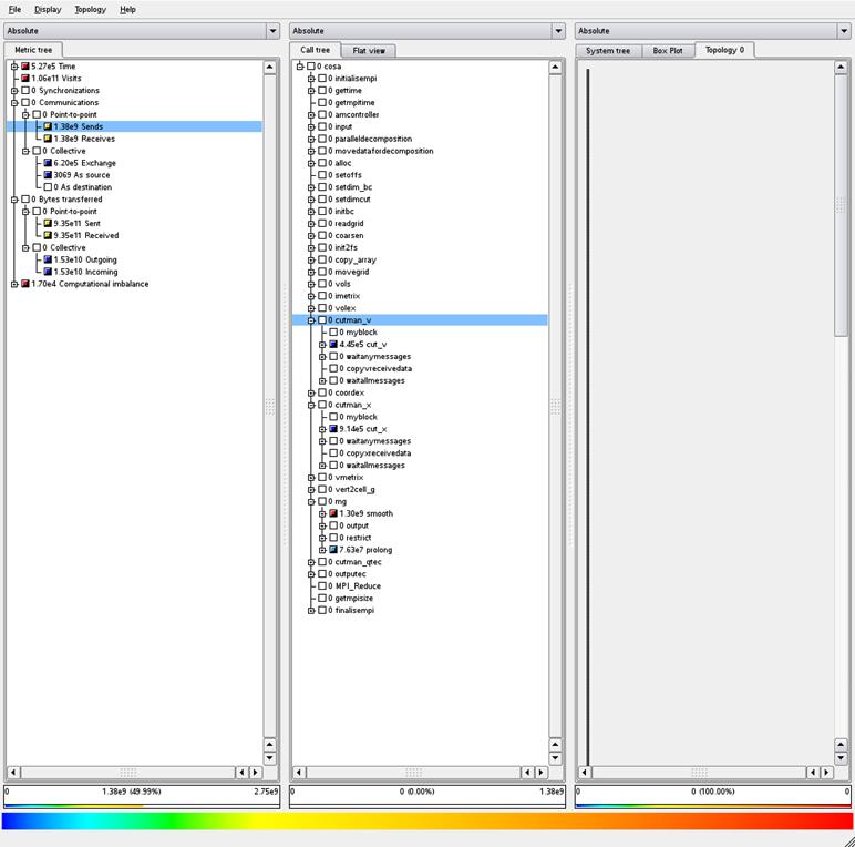
Figure 4: Communications profile, old MPI code using test
case 1
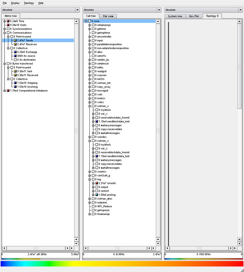
Figure 5: Communications profile, new MPI code using test
case 1
We can see from these Figures that the total amount of data
sent using both versions of the code is exactly the same (see the left hand
column, under the “Bytes transferred” heading).
However, if we look at the “Communications” metric which outlines how
many messages are sent, we can see that the new code sends two orders of
magnitude fewer messages than the old code (1.39 x 10⁹ vs 2.47 x 10⁷
for the sends and receives).
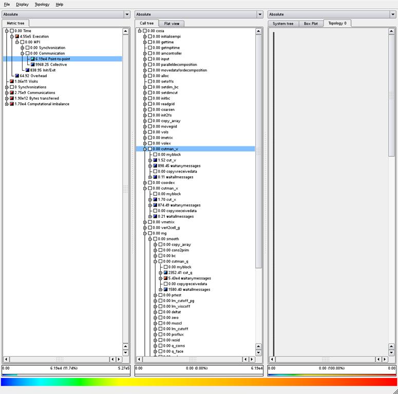
Figure 6: Timings profile, old MPI code using test case 1
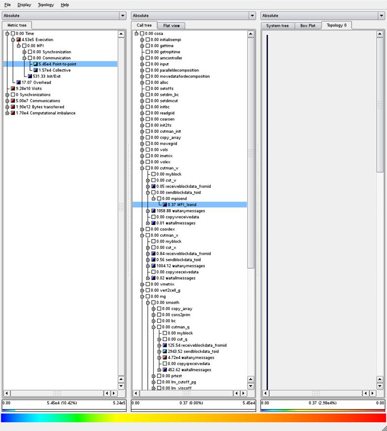
Figure 7: Timings profile, new MPI code using test case 1
Figures 6 and 7 present profile information from the same
runs as Figures 4 and 5, however Figures 6 and 7 now focus on the runtime
information (how much time is spent in routines) rather than how often routines
are called. From these we can see that
the new code does reduce the overall time spent in the messages sent for the halo
exchange (the point-to-point message times are 6.19 x 10⁴ vs 5.45 x
104) however, compared to the overall runtime (approximately 5.2 x
105) this is not a large saving.
Furthermore, the saving in the point-to-point time is balanced by an
increase in the time for the collective communications (from around 1 x 10⁴
for the old code to 1.57 x 10⁴ for the new code).
We can see that optimising the point-to-point communications
when there are collective communications occurring every timestep is simply
moving the place where the synchronisation (and therefore loss of performance)
occurs from the halo communication exchange to the collective (global)
communications. Furthermore, the new MPI
code uses a different approach to the original code. In the original code the halo data associated
with each cut owned by a process is sent as the cut is computed. This means that large numbers of messages are
sent, however it does have the benefit that the communications associated with
sending the cut data are spread out through the cut
calculations/computations. The new code
collects all the data associated with all the cuts a process has to communicate
and then sends them all at once after all the cuts have been processed. This concentrates the communication into a much
smaller section of the code and may cause contention for the communication
network by (as a consequence of the approach taken) meaning processes tend to
all communicate at the same time rather than the communications being spread
out.
However, the performance data we collected was contrary to
what we expected and had experienced on previous versions of HECToR (when COSA
was run on phase2b of HECToR the MPI communications were seen to be more
dominant), therefore we ran the same scaling tests as outlined in Figure 3 on a
different machine (a large Bull supercomputer with 2 x 8 core Intel Xeon
processors per node and an Infiniband QDR interconnect) and collected the
performance data shown in Figure 8.
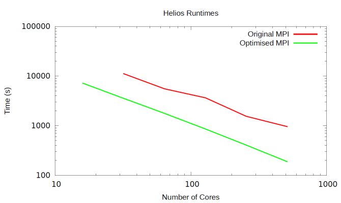
Figure 8: Runtime for the new MPI code vs the old MPI
code on Bull supercomputer using test case 1
We can see from Figure 8 that the performance profile is
significantly different to that of HECToR.
Here, combining the MPI messages has significantly improved the overall
performance at all core counts (it should be noted that we could not complete
the 16 core original MPI job in the time limit for jobs on this machine so it
is not included in the Original MPI line), with the optimised code runtime
being around two orders of magnitude quicker than the original code.
We can, therefore, conclude that the network on HECToR is
very good at performing lots of small messages, so much so that the aggregation
we performed did not significantly improve performance on HECToR. However, for other systems, and even
potentially for ARCHER (depending on what hardware is chosen for that machine),
HECToR’s replacement, this is a very beneficial change.
Following on from the MPI optimisation we documented in the
previous section we looked at the collective communications used within
COSA. The main routine that uses MPI
collective communication functions in COSA is combineforces,
the body of which is outlined below:
do i=1,nbody
temparray(1) = cl(n,i)
temparray(2) = cd(n,i)
datalength = 2
if(functag.eq.3) then
temparray(3) = cm(n,i)
datalength = 3
end if
call
realsumallreduce(temparray,datalength)
cl(n,i) = temparray(1)
cd(n,i) = temparray(2)
if(functag.eq.3) then
cm(n,i) = temparray(3)
end if
end do
Studying this code it is evident that the code is
potentially undertaking more all reduce operations than is necessary,
especially if nbody is large. Furthermore combineforces
is called from within a loop that iterates over the number of harmonics (this
sets the n variable in the code
above), meaning that the all reduce is called nbody*((2*nharms)+1)times.
By moving where combineforces
is called from and aggregating the data to be communicated in the all reduce
operations it is straight forward to combine these all reduce calls into a
single all reduce for each call of the combineforces
routine, as shown below:
j = 1
do k = 0,2*nharms
do i=1,nbody
temparray(j) = cl(k,i)
j = j +1
temparray(j) = cd(k,i)
j = j + 1
temparray(j) = cm(k,i)
j = j + 1
end do
end do
call realsumallreduce(temparray,j-1)
j =
1
do k = 0,2*nharms
do i=1,nbody
cl(k,i) = temparray(j)
j = j +1
cd(k,i) = temparray(j)
j = j + 1
cm(k,i) = temparray(j)
j = j + 1
end do
end do
As with the previous communication aggregation we have
performed this at the expense of extra memory requirements for the combineforces routine, however these
are not significant so do not adversely impact the overall memory footprint of
the code, even for high nbody
and harmonic sizes.
We profiled the new code using scalasca as before, and the
results are shown in Figures 9 and 10
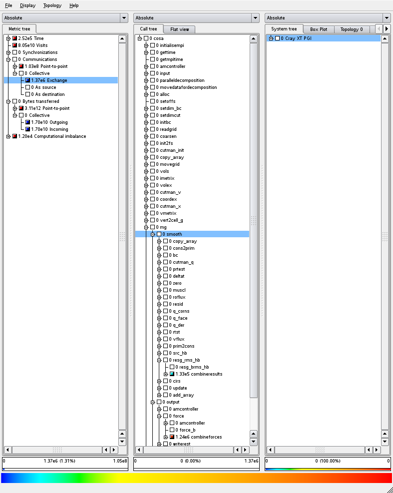
Figure 9: Collective communication profile for the
original MPI code using test case 1
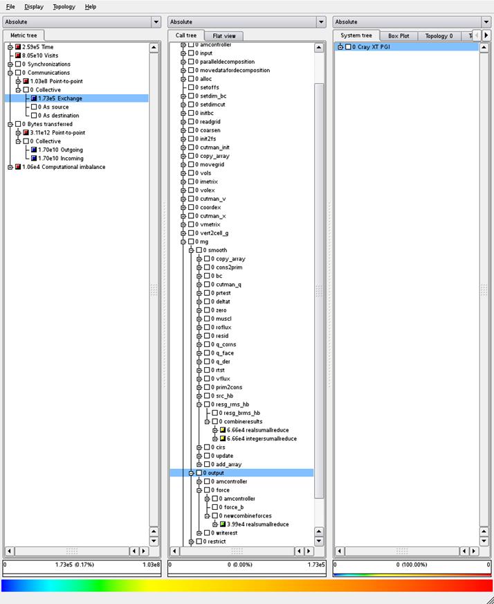
Figure 10: Collective communication
profile for the new MPI code using test case 1
We can see from comparing the number of collective
communications performed in Figures 9 and 10 that the number has reduced by an
order of magnitude, from 1.37 x 10⁶ in Figure 9 to 1.73 x 10⁵
in Figure 10, whilst the amount of data transferred (shown under the bytes transferred section) has stayed
the same.
All the profiling, performance analysis, and optimisation
work we have outlined in the previous sections has been focussing on the main
computational and communication parts of COSA.
Particularly, we have been using COSA with the data output turned
off. However, for any real user of the
code this is not an option, the data that is written into the output files
records the simulation undertaken by the code and enables analysis and
understanding of those simulations.
COSA produces a number of different output files, but for
optimisation there are two types of file that are important, as they are the
largest and require the most time to write; the flowtec files and the restart
file. COSA produces a single restart
file at the end of the simulation (or more frequently if requested by the user)
which can be used to restart the simulation from the point the restart file was
written. It also produces one flowtec
file per real harmonic at the end of the simulation. The flowtec files contain
the solution in a format suitable for use with the commercial CFD postprocessor
and flow visualisation software TECPLOT.
When large simulations are executed the output can be
extremely large, with the restart file being many gigabytes (GB) in size and
each flowtec file being close to a GB in size.
We have noticed when undertaking large simulation with the I/O
functioning that writing these files was taking a significant fraction of the
total runtime.
Therefore, we worked on optimising the I/O used for writing
the main output files to ensure that the I/O is being performed
efficiently. The existing code does use
parallel I/O functionality, calling MPI I/O routines to perform the output from
all processes at once. However, the I/O
is performed, as shown in the example below, through individual writes of data
elements to the file one at a time:
call
setupfile(fid(n),disp,MPI_INTEGER)
call
mpi_file_write(fid(n), 4*doublesize,1,
MPI_INTEGER,MPI_STATUS_IGNORE,ierr)
disp = disp +
integersize
call
setupfile(fid(n),disp,MPI_DOUBLE_PRECISION)
call
mpi_file_write(fid(n),x(i,j,n),1,
&
MPI_DOUBLE_PRECISION,MPI_STATUS_IGNORE, ierr)
disp = disp +
doublesize
call
setupfile(fid(n),disp,MPI_DOUBLE_PRECISION)
call
mpi_file_write(fid(n),y(i,j,n),1,
&
MPI_DOUBLE_PRECISION, MPI_STATUS_IGNORE, ierr)
disp = disp +
doublesize
call setupfile(fid(n),disp,MPI_DOUBLE_PRECISION)
call
mpi_file_write(fid(n),rho,1,
&
MPI_DOUBLE_PRECISION, MPI_STATUS_IGNORE, ierr)
disp = disp +
doublesize
call
setupfile(fid(n),disp,MPI_DOUBLE_PRECISION)
call
mpi_file_write(fid(n),ux,1,
&
MPI_DOUBLE_PRECISION, MPI_STATUS_IGNORE, ierr)
disp = disp +
doublesize
call
setupfile(fid(n),disp,MPI_INTEGER)
call
mpi_file_write(fid(n), 4*doublesize,1,
&
MPI_INTEGER,MPI_STATUS_IGNORE,ierr)
Where the setupfile subroutine
invokes the MPI_FILE_SEEK function.
This use of MPI I/O is not optimal; generally MPI I/O gives
the best performance when large amounts of data are written in a single call to
the file. However, the way the data is
structured in COSA, and the format of the output files, prohibits doing
this.
It is important to the developers and users of COSA that the
output files of the serial and parallel version of the code are the same so in
the scope of this project we did not have the effort to change the way it
currently writes the data. However, we
can optimise the current functionality, aggregating the data to be written into
arrays and then writing that data all at once.
An example of this optimisation of the I/O code outlined above is
provided below:
call
setupfile(fid(n),disp,MPI_INTEGER)
call
mpi_file_write(fid(n), 4*doublesize,1,
&
MPI_INTEGER,MPI_STATUS_IGNORE,ierr)
disp = disp +
integersize
tempdata(tempindex)
= x(i,j,n)
tempindex =
tempindex + 1
tempdata(tempindex)
= y(i,j,n)
tempindex =
tempindex + 1
tempdata(tempindex)
= rho
tempindex =
tempindex + 1
tempdata(tempindex)
= ux
tempindex =
tempindex + 1
call
setupfile(fid(n),disp,MPI_DOUBLE_PRECISION)
call
mpi_file_write(fid(n),tempdata(1),tempindex-1,
&
MPI_DOUBLE_PRECISION, MPI_STATUS_IGNORE, ierr)
disp = disp + doublesize*(tempindex-1)
call
setupfile(fid(n),disp,MPI_INTEGER)
call
mpi_file_write(fid(n), 4*(tempindex-1),1,
&
MPI_INTEGER,MPI_STATUS_IGNORE,ierr)
Testing the new I/O functionality using test case 1 we
collected the following data:
|
|
Runtime (seconds)
|
|
Original MPI Code (No I/O)
|
421
|
|
Original MPI Code
|
701
|
|
New MPI Code
|
547
|
Table 2: I/O functionality runtime
using test case 1
We can see that for the simulation performed (using 512
processes and running for 250 iterations of the simulation) that the original
I/O functionality imposed a significant overhead on the overall simulation
time, increasing the runtime by around 60%.
The optimised I/O functionality reduces this overhead to around 30%,
more than halving the time required to output data to disk. For this simulation the amount of data
outputted is not very large, the restart file is around 350 MB and there are 31
flowtec files of 20 MB each (so overall just less than 1 GB is written to
disk).
However, if we consider a larger simulation then the savings
are even more significant. The previous
simulation (test case 1) had a 512-block grid with 262,144 cells, and 31 real
harmonics, but the simulations currently being studied using COSA typically
have a million or more cells. We
benchmarked the new MPI functionality using test case 3 (which produces a
restart file of around 2.6 GB and 15 flowtec files each 281 MB in size), only
undertaking a single iteration of the simulation. The resultant runtimes on 512 and 2048 cores
are shown in the following table.
|
|
Original I/O Code (seconds)
|
New I/O Code (seconds)
|
|
512 processes
|
1444
|
904
|
|
2048 processes
|
1147
|
801
|
Table 3: Performance of the new I/O
functionality using test case 3
We also discovered a bug in the parallel I/O code when
undertaking this work. When writing very
large restart files (above ~4 GB) the original code did not work. It was ascertained that the code that
calculated the locations in the file for each MPI process to write data to using
a FORTRAN integer datatype. However, on HECToR (and many other machines)
this defaults to a 4-byte integer datatype, and therefore cannot be used to
calculate address bigger than 232 bytes of memory (around 4 GB). We fixed this by specifying these offset
addresses as 8-byte integers in the code, enabling COSA to deal with larger
simulations properly.
We evaluated the overall performance improvement from all
the MPI optimisations we have detailed in this section comparing the
performance of the original code with the latest MPI code, and plotting the
results in Figure 11 below.
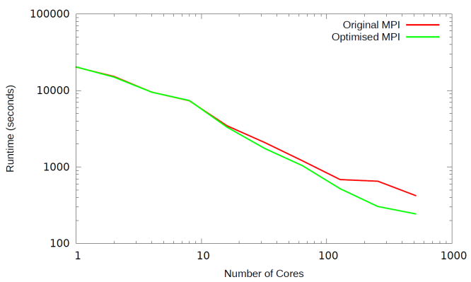
Figure 11: Runtime of the original and
optimised MPI codes using test case 1
We have significantly improved the performance of the code
at larger core counts, with the runtime of the optimised MPI code at 256 and
512 cores around half the time of the original MPI code.
During the performance evaluation of COSA for this project
it was recognised that there were a number of subroutines in the code
implementing standard linear algebra functionality, particularly:
- Matrix inversion
- Matrix-vector products
The harmonic balance Navier-Stokes equations can be viewed
as a set of (2*nharms)+1 steady
problems, all coupled by a source terms depending on the same number of steady
flow solutions, which represent (2*nharms)+1
equally-spaced snapshots of the sought nonlinear periodic flow [2]. The multigrid HB solver of COSA can be
operated in two modes, using either a fully explicit Runge-Kutta (FERK)
smoother, or a Point-Implicit Runge-Kutta (PIRK) smoother. In the PIRK integration, the HB source term is
treated implicitly at each Runge-Kutta stage. This results in the entire
solution update process requiring the solution of ncell linear systems, each of dimension (npde*((2*nharms)+1))at every
Runge-Kutta stage. However, the use of
the PIRK HB integration allows the use of substantially larger pseudo-time
steps for time-marching the solution with respect to the conventional FERK HB
integration, without any loss of numerical stability. As a consequence, a given
convergence level of the HB solution can be achieved using a substantially
lower number of MG iterations using the PIRK rather than the FERK integration.
The original COSA code solved these ncell systems using hand-written linear algebra
routines. These were replaced by the
corresponding routines in the LAPACK and BLAS libraries to ensure that optimal
code for these functions were being used.
All test cases presented in this report used
relatively small time-steps and therefore were run using the FERK HB
integration. However, the PIRK
functionality is now routinely used in production runs of the COSA HB solver,
since it significantly reduces runtimes due to the use of fewer MG cycles. In
order to demonstrate the computational performance improvement achieved by
using the LAPACK routines, test case 1 has been run on HECToR also using the
PIRK HB integration. It has emerged
that, at 512 processes, the new version of the code (using LAPACK routines)
runs in around half the time of the original code (~740 seconds vs ~1400
seconds)
The FERK or PIRK integration are selecting by choosing the
appropriate flag (rkex or rkim) in the input file of COSA.
Using the information obtained in the profiling of the
original code we worked to optimise the OpenMP functionality in COSA. The profiling data shown in Section 2
highlighted the fact that only a small number of routines are heavily used for
harmonic balance simulations.
The original hybrid code, which used the original OpenMP
parallelisation, could be built to parallelise over blocks, harmonics, or grid
cells, depending on the type of simulation being performed. However, as the key strength of COSA is its harmonic
balance functionality we decided to focus the hybrid optimisation on harmonic
balance simulations.
Removing the original OpenMP functionality and
re-implementing OpenMP simply for the key routines we have identified enabled
us to optimise the code by removing OpenMP parallel regions from parts of the
code that are used in the harmonic balance simulations but do not consume much
of the runtime (and therefore do not have enough work within them to justify
the overheads imposed when using OpenMP parallelisations).
The following table contains all the routines in COSA that
had OpenMP added during this work. In
the table the subroutine column lists
those routines that have OpenMP parallel regions in them. The related
subroutines column lists those routines that have orphaned OpenMP do
directives in them which are called by the routines lists in the subroutine column.
|
File
|
Subroutine
|
Related Subroutines
|
|
cosa.f
|
resid
|
bresid
|
|
cosa.f
|
deltat
|
bdeltat
|
|
cosa.f
|
cirs
|
cirs_b
|
|
cosa.f
|
precres
|
prec_bres
|
|
cosa.f
|
src_hb
|
src_bhb
|
|
flux.f
|
roflux
|
roflux_b
|
|
flux.f
|
proflux
|
proflux_b
|
|
flux.f
|
vflux
|
vflux_b
|
|
flux.f
|
muscl
|
muscl_bi
limit_i
muscl_bj
limit_j
|
|
flux.f
|
q_der
|
bq_der_i
bq_der_j
|
|
flux.f
|
rtst
|
b_rtst
|
|
losp.f
|
lsp
|
blsp
|
|
losp.f
|
lm_cutoff_pg
|
lm_bcutoff_pg
|
|
losp.f
|
lm_viscoff
|
lm_bviscoff
|
However, we also recognised that the way the OpenMP code has
been added to COSA also was not efficient.
In general the loops in the code that compute over the harmonics of the
simulation are called within subroutines which are called for each block in the
simulation, and in each subroutine there can be a number of separate loops over
harmonics. Simply parallelising each
harmonic loop with an OpenMP parallel
do directive meant that there were a lot of places that OpenMP parallel
regions were started and finished in the code.
There is an overhead associated with starting and finishing a parallel
region in OpenMP, therefore we re-engineered the OpenMP code we had added to
reduce these overheads.
This reduction in overheads was achieved by hoisting (moving
to a higher level in the program) the parallel regions from within the
subroutines where the harmonic loops are, to the calling subroutine, as shown
in the two code samples in Appendix A.
We also implemented “first touch” initialisation functionality
to ensure that data is initialised on the cores that will be processing
it. The original code zeroed all the
data arrays when they were allocated, and the allocation is done on the master
thread. We have altered the zeroing of
the arrays so it is done in parallel, following the parallelisation pattern
that is used in the rest of the code.
Comparing the performance of the new OpenMP code with that
of the original harmonic OpenMP parallelisation we obtained the scaling data
shown in Figure 12. It should be noted
that this data was collected with I/O turned on, using test case 1, which is
not an ideal test case for the OpenMP harmonic parallelisation.
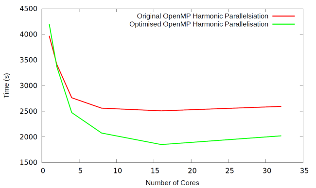
Figure 12: Runtime of the old and new
OpenMP harmonic parallelisation using test case 1
It should also be noted that due to the hardware used in
HECToR, which is AMD Interlagos processors, it is difficult to compare the
performance of 1 process using a single core on a processor to 2 processes
using 2 cores on a processor as the processor is made up of 8 modules, each of
which can run 2 processes (giving the 16 cores in a processor, and HECToR has 2
processor per node giving 32 cores per node), but they share the floating point
unit and memory caches and bandwidth.
The cores can also change their computing frequency if not all the cores
on the processor are being used.
Therefore, the performance of the program using a single core on a processor
(whilst the rest are idle) may be significantly higher than if 2 or more of the
cores are being used as using a single core only potentially gives that process
access to more floating point hardware and memory bandwidth than is available
when 2 processes are running on a module.
This means that calculating the scaling of a parallel code based on the
performance of the code on a single core may not be ideal.
Using this optimised OpenMP implementation improves the
performance of the hybrid code, as shown in the table next, which provides a
comparison of the performance of the hybrid and MPI codes for the old OpenMP
functionality and the optimised functionality (using test case 1).
|
MPI Runtime
|
Old Hybrid Runtime
|
New Hybrid Runtime
|
|
1693
|
2670.13
|
2215.69
|
Table 4: Performance of the hybrid
code using test case 1 on 512 cores
The data in the above table is collected using a simulation
with 512 blocks so the MPI code is using 512 MPI tasks and the hybrid code is
using 128 MPI tasks each with 4 threads.
This means that each MPI task in the hybrid case has 4 blocks of the
simulation, which is not ideal for the performance of the new hybrid code. This hybrid code is designed to work best
when the number of blocks per MPI task is 1, so we also ran the hybrid code
using 512 MPI tasks each with 4 OpenMP threads (using a total of 2048 cores),
the results of which are show in the following table (using test case 1).
|
|
MPI (512 cores)
|
Old Hybrid
(2048 cores)
|
New Hybrid
(2048 cores)
|
|
Runtime (seconds)
|
1693
|
772.16
|
520
|
|
Scaling (compared to the MPI code)
|
N/A
|
2.19
|
3.26
|
Table 5: Performance of the hybrid code
using test case 1 on 2048 cores
We can see that we have improved the performance of the
hybrid code compared to the original hybrid code. However, there is still a performance gap
between the ideal scaling of the hybrid code and the currently scaling of the
hybrid code. Ideally, when using 4 times the number of
cores (as is the case in the example above) the scaling would be 4 times the
pure MPI code, whereas the new hybrid code has a scaling of 3.26.
For the hybrid code we have parallelised the key
computational routines using OpenMP, but as outlined in Section 4 the
performance is still not ideal for the hybrid code. However, there are two areas in the code that
haven’t been parallelised with OpenMP:
The MPI communications are performed over a loop of the cut,
or halo, data. Each cut is independent
so they can be performed by separate threads.
However, as they involve MPI communications then we need to ensure that
we are using the threaded version of the MPI library using the function MPI_INIT_THREAD rather than the usual MPI_INIT function. Furthermore, we need to ensure that the MPI
library being used can support MPI_THREAD_MULTIPLE (individual OpenMP threads can perform MPI
communications).
The I/O undertaken
through the MPI code used MPI I/O functionality. In general the I/O operations are independent
for each block and then each harmonic within the block. However, there are a number of collective
operations (operations that all processes must be involved in) in the I/O
functionality, particularly opening and closing files. To enable the OpenMP threads to be able to
write to the restart and flowtec files independently we needed to ensure that all
the threads are involved in the opening of the files so they each have a
separate file handle to write.
Therefore, we implemented a hybrid file opening and closing strategy as
follows:
!$OMP DO ORDERED
do i=1,omp_get_num_threads()
!$OMP ORDERED
call openfile(fid,'restart',iomode)
!$OMP END ORDERED
end do
!$OMP END DO
Where openfile
calls MPI_FILE_OPEN which is a
collective operations and therefore has to be called from all the OpenMP
threads in the order sequence shown above.
The only other modification that needs to be made to enable file writing
from the OpenMP threads was to ensure that they could correctly calculate where
each harmonic needs to be written to (rather than each block as was the case
previously).
With these optimisations in place the code was once again
benchmarked and the following results collected (using test case 1):
|
|
MPI (512 cores)
|
Original Hybrid
(2048 cores)
|
New Hybrid
(2048 cores)
|
|
Runtime (seconds)
|
1693
|
772.16
|
460
|
|
Scaling (compared to the MPI code)
|
N/A
|
2.19
|
3.68
|
Table 6: Optimised hybrid runtime
using test case 1
We can see that the hybrid code performance has improved,
with close to ideal scaling being obtained for this benchmark case, even when
full functionality (i.e. including I/O) is used. However, it should be noted that to achieve
this performance it is necessary to change the lustre stripe count (which
specifies how many I/O servers can be used to write the file) for the restart
file. By default the restart file has is
setup to use a single I/O server (a stripe count of 1), and this gives ideal
performance of the MPI code and the old hybrid code. However, when the restart I/O functionality
is parallelised with OpenMP the default stripe count does not give ideal performance,
so we changed this stripe count to -1 which enables all available I/O servers
to be used. This gave better performance
than the original stripe count.
The parallelisation of the writing of the flowtec files over
harmonics with OpenMP does not require this as there are multiple flowtec files
which can be distributed to different I/O servers by the lustre file system.
We have undertaken a range of optimisation work on the COSA
simulation code. The MPI optimisation
work we performed has resulted in the new code scaling much better than the
original MPI code, with the overall runtime being reduced to half that of the
original code for a representative test case at 256 and 512 cores on
HECToR. This represents a significant
saving in computational resources.
We have also worked to optimise the hybrid version of the
code. The original hybrid code gave
around a halving in computational runtime for four times the computational
resources, with an operating efficiency of around 55%. The new hybrid code
operates at around 90% efficiency for the same test case on HECToR, again
representing a significant saving in computational resources, and furthermore enabling
users to complete simulations in around half the time that the original code
took for the same problem.
Another outcome of this project is that COSA has now been
installed as a package, available to all users, on HECToR. MPI and hybrid executables are available,
along with a user guide describing the code and how to use it, and example simulations
to enable interested parties to experiment with the software. The executables include all the optimisations
undertaken in this project.
All the code modifications performed in this project have
been incorporated back into the main COSA source code, and extensively tested
to ensure they have not altered the correctness of the COSA simulations.
This work
was supported by Dr M. Sergio Campobasso at Glasgow University.
This
project was funded under the HECToR Distributed Computational Science and
Engineering (CSE) Service operated by NAG Ltd. HECToR – A Research Councils UK
High End Computing Service - is the UK's national supercomputing service,
managed by EPSRC on behalf of the participating Research Councils. Its mission
is to support capability science and engineering in UK academia. The HECToR
supercomputers are managed by UoE HPCx Ltd and the CSE Support Service is
provided by NAG Ltd. http://www.hector.ac.uk
References
[1] M.S.
Campobasso, A. Piskopakis, M. Yan, Analysis of an Oscillating Wing in a
Power-Extraction Regime Based on the Compressible ReynoldsAveraged
Navier-Stokes Equations and the K −ω SST Turbulence Model, ASME
paper GT2013-94531, presented at the ASME/IGTI Turbo Expo 2013 Technical
Conference, 3rd-7th June 2013, San Antonio, Texas, USA..
[2] M.S.
Campobasso and M.H. Baba-Ahmadi, Analysis of Unsteady Flows Past Horizonatal
Axis Wind Turbine Airfoils Based on Harmonic Balance Compressible Navier-Stokes
Equations with Low-Speed Preconditioning, ASME Journal of Turbomachinery,
Vol. 134, no. 6, 2012. DOU: 10.1115/1.4006293.
[3] M.S.
Campobasso and J. Drofelnik, Compressible Navier-Stokes analysis of an
oscillating wing in a power-extraction regime using efficient
low-speed preconditioning, Computers and Fluids, Vol. 67, 2012, pp. 26-40.
DOI: 10.1016/j.compfluid.2012.07.002.
[4] http://www.scalasca.org/
[5] A. Jackson
and M. S. Campobasso. Shared-memory, distributed-memory, and mixed-mode
parallelisation of a cfd simulation code. Computer Science - R&D, 26(3-4):187–195,
2011.
[6] A. Jackson,
M. S. Campobasso, and M. H. Baba-Ahmadi. On the Parallelization of a Harmonic Balance
Compressible Navier-Stokes Solver for Wind Turbine Aerodynamics, pages 747–761.
ASME International, 2011.
Below is an example of the original OpenMP harmonic
parallelisation, including the routine that calls the routine that has been
parallelised.
c---------------------------------------------------------------------
subroutine resid(idir,nl,flux,res)
c---------------------------------------------------------------------
implicit none
include 'common.block'
include 'cosa.inc'
integer*4 idir,nl,iblock,imax,jmax,iflux,ires
real (kind=8) res(*),flux(*)
do iblock = 1,mynblocks
imax
= i_imax (iblock,nl)
jmax
= j_jmax (iblock,nl)
ires
= 1 + off_p3 (iblock,nl) * npde * dim5
iflux
= 1 + off_0 (iblock,nl) * npde *
dim5
call
bresid(flux(iflux),res(ires),idir,imax,jmax,npde,nharms)
end do
return
end
c---------------------------------------------------------------------
subroutine
bresid(flux,res,idir,imax,jmax,npde,nharms)
c---------------------------------------------------------------------
implicit none
include 'common.block'
integer*4 imax,jmax,npde,nharms
integer*4 i,j,idir,ipde,n
real (kind=8)
&
res(-1:imax+1,-1:jmax+1,npde,0:2*nharms),
&
flux(imax,jmax,npde,0:2*nharms)
if (idir.eq.1) then
#ifdef OPENMPNHARMS
!$OMP PARALLEL DO
!$OMP&
PRIVATE(n,ipde,j,i)
!$OMP&
SHARED(nharms,npde,cosa2d,cosa3d,imax,jmax,res,flux)
#endif
do n = 0,2*nharms
do ipde = 1,npde
if
((cosa2d.and.(ipde.ne.4)).or.cosa3d) then
do j = 1,jmax-1
do i = 1,imax-1
res(i,j,ipde,n) =
res(i,j,ipde,n) +
&
flux(i+1,j,ipde,n)-flux(i,j,ipde,n)
end do
end do
end if
end do
end do
#ifdef OPENMPNHARMS
!$OMP END PARALLEL DO
#endif
else if (idir.eq.2) then
#ifdef OPENMPNHARMS
!$OMP PARALLEL DO
!$OMP&
PRIVATE(n,ipde,j,i)
!$OMP&
SHARED(res,flux,cosa3d,npde,nharms,coda2d,imax,jmax)
#endif
do n = 0,2*nharms
do ipde = 1,npde
if
((cosa2d.and.(ipde.ne.4)).or.cosa3d) then
do j = 1,jmax-1
do i = 1,imax-1
res(i,j,ipde,n) =
res(i,j,ipde,n) +
&
flux(i,j+1,ipde,n)-flux(i,j,ipde,n)
end do
end do
end if
end do
end do
#ifdef OPENMPNHARMS
!$OMP END PARALLEL DO
#endif
end
if
return
end
Below is an optimised version of the above routine where the
OpenMP parallel region has been hoisted to the routine above to reduce the
OpenMP overheads.
c---------------------------------------------------------------------
subroutine resid(idir,nl,flux,res)
c---------------------------------------------------------------------
implicit none
include 'common.block'
include 'cosa.inc'
integer*4
idir,nl,iblock,imax,jmax,iflux,ires
real (kind=8) res(*),flux(*)
#ifdef OPENMPNHARMS
!$OMP PARALLEL
DEFAULT(NONE)
!$OMP&
SHARED(mynblocks, i_imax, j_jmax, off_p3, off_0, nharms, nl, npde, dim5)
!$OMP& SHARED(flux,
res, idir)
!$OMP& PRIVATE(imax,
jmax, ires, iflux, iblock)
#endif
iblock = 1,mynblocks
imax
= i_imax (iblock,nl)
jmax
= j_jmax (iblock,nl)
ires
= 1 + off_p3 (iblock,nl) * npde * dim5
iflux
= 1 + off_0 (iblock,nl) * npde *
dim5
call
bresid(flux(iflux),res(ires),idir,imax,jmax,npde,nharms)
end do
#ifdef OPENMPNHARMS
!$OMP END PARALLEL
#endif
return
end
c---------------------------------------------------------------------
subroutine
bresid(flux,res,idir,imax,jmax,npde,nharms)
c---------------------------------------------------------------------
implicit none
include 'common.block'
integer*4 imax,jmax,npde,nharms
integer*4 i,j,idir,ipde,n
real (kind=8)
&
res(-1:imax+1,-1:jmax+1,npde,0:2*nharms),
&
flux(imax,jmax,npde,0:2*nharms)
if (idir.eq.1) then
#ifdef OPENMPNHARMS
!$OMP DO
!$OMP&
PRIVATE(n,ipde,j,i)
#endif
do n = 0,2*nharms
do ipde = 1,npde
if
((cosa2d.and.(ipde.ne.4)).or.cosa3d) then
do j = 1,jmax-1
do i = 1,imax-1
res(i,j,ipde,n) =
res(i,j,ipde,n) +
&
flux(i+1,j,ipde,n)-flux(i,j,ipde,n)
end do
end do
end if
end do
end do
else if (idir.eq.2) then
#ifdef OPENMPNHARMS
!$OMP DO
!$OMP&
PRIVATE(n,ipde,j,i)
#endif
do n = 0,2*nharms
do ipde = 1,npde
if
((cosa2d.and.(ipde.ne.4)).or.cosa3d) then
do j = 1,jmax-1
do i = 1,imax-1
res(i,j,ipde,n) =
res(i,j,ipde,n) +
&
flux(i,j+1,ipde,n)-flux(i,j,ipde,n)
end do
end do
end if
end do
end do
end if
return
end
The
configuration data for each of the test cases is included below.
*** input file for 2D Euler/NS COSA solver ***
model
id flow-type debug
laminar
1 external n
gamma
reyno pranl machfs
alpha
1.4d0
1100 0.71d0 1.d-01
0.d0
flow-mode
solver rk option nharms
freq.
unsteady
hb rkex 15
0.014
move
dh0x dh0y xh yh
dthet0 phipp
plupit
0.d0 1.d0 0.33333333 0.d0 76.33d0 270.d0
irest
srest cfl lmax
iupdt toler
0 1500 0.5
250 1 1.d-20
rkap
irs-typ cfli psi
-1.
cirs_v1 1.0 0.25
ilim
epslim cntrpy etpfxtyp entfxctf
0
5.d-04 0.d0 0
0.95d0
nlevel
nl_crs nl_fmg nstart
npre npost ncrs
3
2 1 5 5
5 10
prol. type
bilinear
flow-speed
nolomach
tref
288.2
functional
cl_cd_cm_1 0.33333333 0.0
1
20 475 476 479 480 483 484 487 488 491 492 495 496
499 500 503 504 507 508 511 512
512
Coarse input file:
*** input file for 2D Euler/NS COSA solver ***
model
id flow-type debug
laminar
1 external n
gamma
reyno pranl machfs
alpha
1.4d0
1000 0.71d0 0.2244
9.138
flow-mode
solver rk option nharms
freq.
unsteady
hb rkex 8
0.002707149187620
move
dh0x dh0y
plunge
1.2091 0.d0
irest
srest cfl rmpf
lmax iupdt toler
0 4000 1.5
1.0 10000 1
1.d-13
rkap
irs-typ resper cfli
psi
-1.
cirs_v1 0 3.0d0 0.25
ilim
epslim cntrpy etpfxtyp
entfxctf
0
5.d-04 0.d0 0 0.95d0
nlevel
nl_crs nl_fmg nstart
npre npost ncrs
3
4 1 2 2
2 8
flow-speed cff-typ
visc-prec prec-typ lx ly
lomach 2
viscous mixed 28.0
28.0
epsp(1)
epsp(2) epsp(3)
2.d-1
9.d-1 9.d-1
tref
288.2
functional
clmom 0.25d0 0.d0
1 !
nbody
12 3 4
5 6 7 8 9
10 11 12
13 14 ! n_bodblo, i_bdbl(i_bodblo)
32
Fine input file:
*** input file for 2D Euler/NS COSA solver ***
model
id flow-type debug
laminar
1 external n
gamma
reyno pranl machfs
alpha
1.4d0
1000 0.71d0 0.2244
9.138
flow-mode solver rk option
nharms freq.
unsteady
hb rkex 8
0.002707149187620
move
dh0x dh0y
plunge
1.2091 0.d0
irest
srest cfl rmpf
lmax iupdt toler
0 4000 1.5
1.0 10000 1
1.d-13
rkap
irs-typ resper cfli
psi
-1.
cirs_v1 0 3.0d0 0.25
ilim
epslim cntrpy etpfxtyp
entfxctf
0
5.d-04 0.d0 0 0.95d0
nlevel
nl_crs nl_fmg nstart
npre npost ncrs
3
4 1 2 2
2 8
flow-speed cff-typ
visc-prec prec-typ lx ly
lomach
2 viscous mixed
28.0 28.0
epsp(1)
epsp(2) epsp(3)
2.d-1
9.d-1 9.d-1
tref
288.2
functional
clmom 0.25d0 0.d0
1 !
nbody
12 27 25
23 21 19 18 3
4 5 7
9 11 ! n_bodblo, i_bdbl(i_bodblo)
32
*** input file for 2D Euler/NS COSA solver ***
model
id flow-type debug
laminar
1 external n
gamma
reyno pranl machfs
alpha
1.4d0
1000 0.71d0 0.2244
9.138
flow-mode
solver rk option nharms
freq.
unsteady
hb rkex 8
0.002707149187620
move
dh0x dh0y
plunge
1.2091 0.d0
irest
srest cfl lmax
iupdt toler
0 200 1.5 2
1 1.d-12
rkap
irs-typ cfli psi
-1.
cirs_v1 3.0d0 0.25
ilim
epslim cntrpy etpfxtyp entfxctf
0
5.d-04 0.d0 0 0.95d0
nlevel
nl_crs nl_fmg nstart
npre npost ncrs
3
4 1 2 2
2 8
prol. type
bilinear
flow-speed cff-typ
visc-prec prec-typ lx ly
lomach
2 viscous mixed
28.0 28.0
epsp(1)
epsp(2) epsp(3)
2.d-1
9.d-1 9.d-1
tref
288.2
functional
cl_cd_cm_0 0.25d0 0.d0
1
48 9 10 11 12 13 14 15 16 17 18 19 20 21 22 23 24
25 26 27 28 29 30 31 32 33 34 35 36 37 38 39 40 41 42 43 44 45 46 47 48 49 50
51 52 53 54 55 56
2048