Adding Spin Polarisation and van der Waals Energy Correction to Conquest
\( \newcommand{\up}{\uparrow} \) \( \newcommand{\dn}{\downarrow} \) This report describes the work done in the distributed Computational
Science and Engineering (dCSE) project aimed to extend functionality
of the linear scaling ab initio Density Functional Theory code
Conquest by adding spin polarisation and van der Waals functional
described by works of Dion et al.[3] and Roman-Perez et
al.[15]. This work would allow Conquest to
perform simulations on magnetic systems and on bio-molecular systems
in which van der Waals interactions are essential. The
implementations has been successful.
Table of Contents
- 1 Introduction
- 2 Implementing Spin Polarisation
- 3 Implementing van der Waals Energy Correction
- 4 Conclusion and Future Work
- 5 Acknowledgement
1 Introduction
There are various classes of important problems in biochemistry which rely quantum mechanical properties of the biological systems dominate. Due the complexity of biomolecules and the importance of environment (such as the presence of water), isolated quantum mechanical studies on a small part of the molecule may not be sufficient in reproducing and understanding the key properties of the molecule. The ideal quantum mechanical method would allow simulation of a large part of the biomolecule (or even the entire molecule) inside an environment in a highly scalable manner on modern high performance computation platforms. The method should also correctly model the systems which contain transition metal complexes and van dar Waals interactions.
Conquest is a linear scaling Density Functional Theory (DFT) code
which has demonstrated excellent scaling for computation on large
number of cores. The good scaling makes it an appealing platform
for large scale quantum mechanical studies on biomolecules. The aim
of this dCSE project is to extend the infrastructure of Conquest
to include spin polarisation, and to incorporate a first principle
density functional for van der Waals interactions[3].
This project aims to add the collinear form of spin polarisation
into Conquest. This means there are two spin states (\(\up\) and
\(\dn\)). Conquest was originally written for spin non-polarised
calculations only, and the data structures in the code reflect
this. For this reason a significant portion of the code has to be
updated to accommodate the extra degrees of freedom introduced by
spin. Never-the-less, linear scaling is generally not effected by
adding spin. This is because the spin implementation always uses
the existing Conquest kernels for distributing data and
computation, so the underlying communication and computation
mechanisms have not been changed. Since the implementation of spin
spreads through-out the code and involves some changes to data
structure while the van der Waals functional can be written within
additional modules and uses spin dependent quantities, it was
decided that spin implementation should be done before the work on
van der Waals functional.
There are two flavours of spin polarised calculation implemented for this project:
- Calculations with spin populations fixed to user given values through-out.
- Calculations that start with spin populations set by the user, but then are allowed to change—while still keeping the total electron number fixed—and self-adjust to give minimum energy. The final difference of the spin populations will be the relaxed spin polarisation of the system.
In contrast to the implementation of spin polarisation, van der Waals functional can be implemented as a relatively self-contained module. The implementation follows closely to the work done by Dion et al.[3] and Roman-Perez et al.[15].
This report describes the work done for implementing the updates to
Conquest mentioned above. Since this work is oriented around
extending features and functionality of the code, most resources
has been allocated to code development rather than profiling and
optimisation. For work on spin since large parts of the code has
been updated, and most involve simply adding a loop in the
calculation for the second spin component. It would be impractical
and tedious to include in this report all the changes made to the
code. I will therefore only give an account of the relatively
important parts of the modification.
2 Implementing Spin Polarisation
Conquest before the project started only handles spin
non-polarised calculations. This means that only the matrices and
grid data associated to one spin component are stored and
calculated, and any extensive quantities are calculated with an
additional factor of 2 knowing the contribution from spin up and
down components are identical. The aim of this dCSE project is to
extend this to allow collinear1 spin polarisation calculations,
where physical quantities associated to each spin channels (\(\up\)
and \(\dn\)) are calculated and are allowed to differ with the
constraint that total number of electrons has to be conserved.
Conquest uses a set of optimised support functions as a basis-set
to give matrix representations of the various quantum mechanical
operators. The support functions them-selves are generated by using
linear combination of a set of basis functions either in the
form of psudo-atomic orbitals (PAOs) or localised blip (B-spline)
functions[2]. Each support function centers on a given
atom and only basis functions within a given range contributes to
the support function. This ensures strict locality of the support
functions and hence making linear-ordering calculations possible.
The coefficients of the linear combinations are then optimised
during the energy minimisation step to ensure the minimum energy is
found with the given set of basis functions.
Ideally for spin polarised calculations, in addition to separate
matrices and data on grid for physical quantities in each spin
channel, one would also benefit from making the support functions
them-selves spin dependent. This offers more flexibility in
optimising the basis coefficients and hence leads to more optimised
ground-state energies. However allowing the support functions to be
spin dependent would mean rewriting a significant portion of
Conquest given virtually all subroutines and quantities in the
code except the core linear algebra, FFT and MPI communication
kernels depend or operate on the support functions and their derived
quantities. Therefore within the given time-frame of the project, we
have decided to use the existing support functions in Conquest for
both spin channels.
2.1 Changes To Data Structure
There are in general three types of data storage for physical
quantities in Conquest:
- Matrices: These store the overlap of the support functions and
matrix representations of the quantum operators in a compressed
(sparse) format and distributes them to processors with respect
to the atomic labels in rows.
Conqueststores the matrices in a stack and refers to each matrix using an unique integer tag. - Functions-on-grid: These store the support functions
them-selves and Kleinman-Bylander (K.B.) non local pseudopotential
projectors (including those linearly operated by a matrix), which
are functions of a given label (be it support function label or
KB projector label) defined on every grid point.
Conquestdistributes these functions according to the real-space grid point blocks, so that each processor gets a subset of such functions (with values associated to all atomic and support labels) on a set of real-space grid points (organised in blocks) it is in charge of. Again the data associated to the functions are stored in a stack and there is an unique integer tag referring to each function. Note that the set of all support functions is considered to be a single "function on grid". - Numbers-on-grid: These store the function of the form
\(f(\vec{r})\) defined on the real-space or FFT grid. They differ
from "functions on grid" in that there is no other index
dependencies other than that associated to the grid point. These
are stored as ordinary arrays of real numbers.
Conquestdistributes them among the processors again according to the real-space grid point blocks.
For collinear spin polarised calculations the matrices are given as direct sums of its spin components: \begin{equation*} \mat{M} = \mat{M}^\up \oplus \mat{M}^\dn \equiv \begin{pmatrix} \mat{M}^\up & 0 \\ 0 & \mat{M}^\dn \end{pmatrix} \end{equation*} Hence the matrices have the properties: (\(\alpha, \beta \in \mathbb{C}\)) \begin{align*} (\alpha\mat{A} + \beta\mat{C})\mat{B} = \bigl( (\alpha\mat{A}^\up + \beta\mat{C}^{\up}) \mat{B}^\up \bigr) \oplus \bigl( (\alpha\mat{A}^\dn + \beta\mat{C}^{\dn}) \mat{B}^\dn \bigr) \end{align*}
The following global matrices in Conquest are spin dependent:
| Matrix | Conquest Variable | Description |
| \(\mat{L}\) | matL | auxiliary matrix, all indices contravariant |
| \(\mat{K}\) | matK | density matrix, all indices contravariant |
| \(\mat{H}\) | matH | Hamiltonian matrix, all indices covariant |
| \(\mat{L}\mat{S}\) | matLS | auxiliary matrix, second index covariant |
| \(\mat{S}\mat{L}\) | matSL | auxiliary matrix, first index covariant |
| \(\mat{\Phi}\) | matphi | derivative of electron no. w.r.t. auxiliary matrix |
| \(\mat{M}_{12}\) | matM12 | part of derivative of energy w.r.t. support functions |
| \(\mat{M}_{4}\) | matM4 | part of derivative of electron no. w.r.t. support functions |
All of these matrices were originally implemented in Conquest as
integer variables storing the tag to the internal matrix stack. For
spin polarised calculations, we need a second copy for the other
spin component. We also need to make sure that there will be no
memory wastage when doing spin non-polarised calculations and only
one set of the above matrices are allocated and used. The easiest
way to achieve this is to add a global control variable nspin
which can be either 1 for spin non-polarised calculations or 2 for
spin polarised calculations. Then the matrices in the above list
(and all other similar matrices used as local variables within
subroutines) are redefined as allocatable integer arrays of
dimension nspin. Hence once allocated and initialised at the
beginning of execution, matM(1) corresponds to \(\mat{M}^\up\) and
matM(2) corresponds to \(\mat{M}^\dn\).
Conquest was not consistent in the definition of the spin
non-polarised matrices in its original implementation. For example,
matL and matH were defined as \(\mat{L}^\up\) and \(\mat{H}^\up\)
correspondingly, however matphi was defined as \(2 \mat{\Phi}^\up =
\sum_\sigma \mat{\Phi}^{\sigma}\) (\(\sigma\) denotes spin). To be
consistent and avoid future confusion—that leads to bugs, I
modified this definition so that matM(1) always refers to the
spin up component of the matrix \(\mat{M}\) irrespective to whether
the calculation is spin polarised or not.
As we have discussed in section Implementing Spin Polarisation the overlap matrix \(\mat{S} = S_{i\alpha j\beta} = \braket{\phi_{i\alpha}}{\phi_{j\beta}}\)—where \(\phi_{i\alpha}(\vec{r})\) are the support functions—is treated as spin independent.
Extensive quantities such as the energy and electron numbers are
calculated as traces of spin dependent matrices. The trace of any
matrix \(\mat{M}\) is simply the sum of the trace of its spin
components:
\begin{equation*}
\tr{\mat{M}} = \tr\mat{M}^\up + \tr\mat{M}^\dn
\end{equation*}
To take into account that only one of the spin component is stored
for spin non-polarised calculations, I have introduced a factor
spin_factor which is set to 1.0 for spin polarised calculations
and 2.0 otherwise. so that the above sum is performed in the code
as follows:
value = zero
do spin = 1, nspin
  value = value + spin_factor * trace(matM(spin))
end do
Conquest stores three functions-on-grid as global variables
available through using functions_on_grid module. They correspond
to the support functions, the result of Hamiltonian matrix acting
on the support functions (H_on_support) and the pseudopotential
functions. Only H_on_support should be spin dependent as the
Hamiltonian matrix is spin dependent. Therefore following the same
method for matrices, I redefined the integer variable
H_on_support (which stores the tag referencing the
functions-on-grid object in the internal stack) as an array of
dimension 2. Because of the way the functions on grid reference
tags are implemented, it would be difficult to allow the dimension
of H_on_support to vary according to value of nspin. However to
save memory for non-spin polarised calculations, there will still
only one functions-on-grid object allocated in the stack for
H_on_support and only H_on_support(1) references to the correct
location in the stack.
Spin dependent numbers-on-grid global quantities in Conquest are
density, and potential, both are redefined as allocatable real
arrays of dimension (maxngrid, nspin). maxngrid stores the
maximum number of grid points on the node. Again to avoid
confusion, density(1) always stores the electron density for the
spin up channel irrespective to whether the calculation is spin
polarised or not. The original Conquest had a factor of 2
contained inside density so that it gives the total density. This
has been redefined after the spin implementations.
2.2 Order \(N\): Spin Polarised Energy Minimisation
Under linear scaling scheme, Conquest finds the ground-state
energy of a system by minimising band-energy:
\begin{equation*}
E = \tr(\mat{H}\mat{K}) = \sum_\sigma\tr(\mat{H}^{\sigma}\mat{K}^{\sigma})
\end{equation*}
by varying the auxiliary matrices \(\mat{L}^{\sigma}\) under the
constraint on the conservation number of electrons. The density
matrix \(\mat{K}^{\sigma}\) is defined in terms of the auxiliary and
overlap matrices
\begin{equation*}
\mat{K}^{\sigma}
= 3\mat{L}^{\sigma}\mat{S}\mat{L}^{\sigma} -
2\mat{L}^{\sigma}\mat{S}\mat{L}^{\sigma}\mat{S}\mat{L}^{\sigma}
\end{equation*}
The minimisation is an iterative process by working out a search direction based on the gradient of the energy with respect to \(\mat{L}^\sigma\); propagate the auxiliary matrix along the search direction until a local minimum is found; and a new search direction is worked out from there and repeat the process. At \(n + 1\)-th step, the auxiliary matrix (written as a direct sum) may be written as \begin{equation*} \mat{L}_{n+1} = \mat{L}_n + \lambda_n \mat{G}_n \end{equation*} For spin polarised calculations we treat the problem as a minimisation procedure on the direct sum of the spin dependent matrices.
The search direction \(\mat{G}_n = \mat{G}^\up_n \oplus \mat{G}^\dn_n\) is calculated to be the direction opposite to the slope in energy surface \(\pdiff{E}{\mat{L}^{\sigma}}\) and then corrected so that it remains on the tangent plane to the iso-electron-number surface. The step \(\lambda_n\) is calculated by minimising E along \(\mat{G}_n\).
There are two choices for the search direction, which in turn define the type of problem we wish to calculate.
- The spin populations (i.e. total magnetisation) are fixed. In this case the search direction in each spin channel is corrected so that the it stays on the tangent plane of the iso-electron-number surface for the particular spin: \begin{align*} \mat{G}_n^\up & = - \pdiff{E}{\mat{L}^\up} + \frac{ \left( \pdiff{E}{\mat{L}^\up} \cdot \pdiff{N}{\mat{L}^\up} \right) }{ \Norm{\pdiff{N}{\mat{L}^\up}}^2 } \pdiff{N}{\mat{L}^\up} \\ \mat{G}_n^\dn & = - \pdiff{E}{\mat{L}^\dn} + \frac{ \left( \pdiff{E}{\mat{L}^\dn} \cdot \pdiff{N}{\mat{L}^\dn} \right) }{ \Norm{\pdiff{N}{\mat{L}^\dn}}^2 } \pdiff{N}{\mat{L}^\dn} \end{align*}
- The spin populations are allowed to vary, but the total electron number \(N = N^\up + N^\dn\) are required to be fixed. In this case the search direction is corrected so that the direct sum \(\mat{G}\) needs to stay on the tangent plane \(\pdiff{N}{\mat{L}}\) of the iso-surface of the total electron number. Hence \begin{align*} \mat{G}_n^\up & = - \pdiff{E}{\mat{L}^\up} + \frac{ \left( \pdiff{E}{\mat{L}} \cdot \pdiff{N}{\mat{L}} \right) }{ \Norm{\pdiff{N}{\mat{L}}}^2 } \pdiff{N}{\mat{L}^\up} \\ \mat{G}_n^\dn & = - \pdiff{E}{\mat{L}^\dn} + \frac{ \left( \pdiff{E}{\mat{L}} \cdot \pdiff{N}{\mat{L}} \right) }{ \Norm{\pdiff{N}{\mat{L}}}^2 } \pdiff{N}{\mat{L}^\dn} \end{align*} where \(\pdiff{E}{\mat{L}} \cdot \pdiff{N}{\mat{L}} \equiv \pdiff{E}{\mat{L}^\up} \cdot \pdiff{N}{\mat{L}^\up} + \pdiff{E}{\mat{L}^\dn} \cdot \pdiff{N}{\mat{L}^\dn}\) and \(\pdiff{N}{\mat{L}} \cdot \pdiff{N}{\mat{L}} \equiv \pdiff{N}{\mat{L}^\up} \cdot \pdiff{N}{\mat{L}^\up} + \pdiff{N}{\mat{L}^\dn} \cdot \pdiff{N}{\mat{L}^\dn}\).
Note that in Conquest \(\pdiff{N}{\mat{L}}\) is named as \(\mat{\Phi}\) and
stored in matphi. And the dot product \(\mat{A} \cdot \mat{B}\)
between matrices is defined as trace of their product
\(\tr(\mat{A}\mat{B})\) and norm of a matrix is defined as the square
root of its own dot product \(\norm{\mat{A}} = \sqrt{\mat{A} \cdot
\mat{A}}\).
The difference in the definition of search direction is crucial for calculations where spin is allowed to vary, because the constraint on total electron number means electron populations within each channel are allowed to readjust, whereas the definition of \(\mat{G}\) in the first case (fixed spin population) prohibits this.
Special attention should be paid to the "step-size" \(\lambda_n\). While for spin polarised case it is possible to make \(\lambda_n = \lambda_n^\sigma\) to be spin dependent, it is important to bear in mind that each minimisation step is should be a linear propagation of the auxiliary matrix (direct sum of the spin components), and making the propagation step spin dependent breaks this linearity.
2.2.1 Pulay Minimisation
To find the minimum band energy the procedure \(\mat{L}_{n+1} +
\lambda_n \mat{G}_n\) is repeated until \(\mat{G}\) becomes less than
a given tolerance. One can readily see that this procedure is
identical to the linear mixing method used for calculating
self-consistent densities. This means we can employ the Pulay
methods[14][6] for making the minimisation
faster. Conquest implements this by regarding \(\mat{G}\) as the
residual.
The key to extending the implementation to spin polarised calculations is to understand that the minimisation process sees the over all direct sum of the spin matrices as the minimisation variable, not its individual spin components. Therefore the correct form to use for magnitude for the residual is given as \(\norm{\mat{G}}\), or for more simplicity \(\norm{\mat{G}}^2 = \tr(\mat{G}\mat{G}) = \sum_\sigma \tr(\mat{G}^\sigma\mat{G}^\sigma)\). Because the Pulay minimisation procedure concerns the direct sum matrix, there is no difference to whether the spin population is fixed or not. The different constraints on electron number are included in the definition of \(\mat{G}^{\sigma}\).
2.2.2 Constraint on Electron Numbers
While the definition of the search directions ensures the new
auxiliary matrices stay on tangent plane of the iso-electron
number energy surfaces, this still only conserves the electron
numbers up to the first order. It was found that the accuracy and
stability of ground-state energy calculations are highly dependent
on electron numbers being correct at each minimisation iteration
step. Hence Conquest employs a further step to correct
\(\mat{L}\) to give the correct number of electrons.
For spin polarised calculations things are slightly more
complex. For the case of fixed spin populations, we want to apply
electron number corrections so that populations in each spin
channels remain the same as those at the beginning of the
calculation. On the other hand for spin relaxation calculations,
we would need to allow the electron populations in each spin
channels to vary while keeping the total electron number the
same. The spin non-polarised calculations are in effect the same
as spin-fixed calculations with same populations in each channel,
and therefore it is easy to convert the existing electron number
correction subroutine in Conquest to work with both spin
non-polarised and fixed polarisation cases. For spin relaxation
calculations, a new subroutine has to be written.
The basic idea behind the procedure for electron number correction is to find the correct step-size \(x\) along a search direction so that \begin{equation*} \mat{L}' = \mat{L} + x \mat{\Gamma} \end{equation*} gives the correct number of electrons. For spin-fixed or non-spin polarised case, this means we need to find \(x^\sigma\) for each spin channel \(\sigma\) (for spin non-polarised calculations we of course only need to correct electron number for one spin channel as the other is assumed to be identical), so that \begin{equation*} N(\mat{L}'^\sigma) = \tr(3\mat{S}\mat{L}'^{\sigma}\mat{S}\mat{L}'^\sigma) - \tr(2\mat{S}\mat{L}'^{\sigma}\mat{S}\mat{L}'^\sigma\mat{S}\mat{L}'^\sigma) = N^\sigma \end{equation*} where \(N^\sigma\) are the spin populations defined by user at initialisation. For spin relaxation calculations, we should treat the electron correction process as an linear operator acting on the direct sum \(\mat{L}\), so that the step \(x\) should not be spin dependent. We need to find \(x\) so that \begin{equation*} \sum_\sigma N(\mat{L}'^\sigma) = \sum_\sigma \left( \tr(3\mat{S}\mat{L}'^{\sigma}\mat{S}\mat{L}'^\sigma) - \tr(2\mat{S}\mat{L}'^{\sigma}\mat{S}\mat{L}'^\sigma\mat{S}\mat{L}'^\sigma) \right) = N \end{equation*} where \(N\) is the total number of electrons in the system under calculation.
Since the energy minimisation step takes \(\mat{L}\) slightly away from the iso-electron number surface, the search direction thus should be perpendicular to that surface. This means \begin{equation*} \mat{\Gamma}^\sigma = \mat{S}^{-1} \pdiff{N^\sigma}{\mat{L}^{\sigma}} \mat{S}^{-1} \equiv \mat{S}^{-1} \mat{\Phi}^\sigma \mat{S}^{-1} \end{equation*} where \(N^\sigma = N(\mat{L}^{\sigma})\), and the inverse of overlap matrix appears because the support functions are non-orthogonal. Note that because electron number is an extensive quantity and \(N(\mat{L}) = N(\mat{L}^\up) + N(\mat{L}^\dn) = N^\up + N^\dn\), \(\pdiff{N}{\mat{L}^\sigma} = \pdiff{N^\sigma}{\mat{L}^\sigma}\) so that the search direction is the same for both fixed spin and spin relaxation calculations.
The step size \(x\) (or \(x^\sigma\) for fixed spin or non-polarised case) is calculated by recognising that \(N(\mat{L} + x\mat{\Gamma})\) is a cubic polynomial of \(x\), and \(x\) (or \(x^\sigma\)) needs to be chosen so that \(N\) (or \(N^\sigma\)) is stationary—that is its derivative with respect to \(x\) is zero.
The electron number correction procedure is done after every Pulay energy minimisation step to ensure the electron numbers are correct through out minimisation process.
2.3 Order \(N\): McWeeny Initialisation
For order \(N\) calculations, before entering the energy minimisation procedures, the auxiliary matrices are first initialised to make sure its eigenvalues are in between 0 and 1. It is then passed through a McWeeny iteration loop[8][1] so that all of the eigenvalues of \(\mat{L}\) are either 0 or 1. This ensures idempotency of the density matrix, and hence conservation of electron number.
The McWeeny initialisation and iteration procedures used by
Conquest is described by the works of Palser and
Manolopoulos[8], and extended to non-orthogonal basis
sets (support functions) by Bowler[1].
2.3.1 Case for Fixed Spin Populations
To extend the procedure for spin polarised calculations, I noted again that the fixed spin case is equivalent to spin non-polarised case, one only has to repeat the original procedures for the other spin channel. The initial guess for the \(\sigma\) channel auxiliary matrix thus should be given as \begin{equation*} \mat{L}_0^\sigma = \frac{\lambda^\sigma}{N} \left( \mu^\sigma \mat{S}^{-1} - \mat{S}^{-1} \mat{H}^{\sigma} \mat{S}^{-1} \right) + \frac{N^\sigma_e}{N} \mat{S}^{-1} \end{equation*} where \(N\) is the dimension of \(\mat{L}^{\sigma}\) matrix, which equals to the total number of support functions available for the calculation. \(N_e^\sigma\) is the fixed population for spin channel \(\sigma\), and \begin{equation*} \lambda^\sigma = \min\left( \frac{N^\sigma_e}{H^\sigma_{\text{max} - \mu^\sigma}}, \frac{N - N^\sigma_e}{\mu^\sigma - H^\sigma_{\text{min}}} \right) \end{equation*} where \(H^\sigma_{\text{max}}\) and \(H^\sigma_{\text{min}}\) are bounds to the maximum and minimum eigenvalues of the Hamiltonian component in spin channel \(\sigma\).
\(\mu^\sigma\) takes values depending on the value of \begin{equation*} \mu^\sigma = \begin{cases} \frac{\tr(\mat{S}\mat{S}^{-1}\mat{H}^\sigma\mat{S}^{-1})}{N} + A H^\sigma_{\text{max}} & \text{if} \quad H^\sigma_{\text{min}} < \mu^\sigma < H^\sigma_{\text{max}} \\ \frac{\frac{\tr(\mat{S}\mat{S}^{-1}\mat{H}^\sigma\mat{S}^{-1})}{N} - \frac{AN^\sigma_eH^\sigma_{\text{min}}}{N - N^\sigma_e}} {1 - \frac{AN}{N - N^\sigma_e}} & \text{if} \quad H^\sigma_{\text{min}} < \mu^\sigma < H^\sigma_{\text{max}} \end{cases} \end{equation*} \(A\) is the "error" which comes from the fact that \(\mat{S}^{-1}\) is not exact for order \(N\) calculations: \(A = 1 - \frac{\mat{S}\mat{S}^{-1}}{N}\).
The McWeeny iteration step is given as: \begin{equation*} \mat{L}^{\sigma}_{n+1} = \begin{cases} \frac{(1 - 2c^\sigma_n)\mat{L}^{\sigma}_n + (1 + c^\sigma_n)\mat{L}^{\sigma}_n\mat{S}\mat{L}^{\sigma}_n - \mat{L}^{\sigma}_n\mat{S}\mat{L}^{\sigma}_n\mat{S}\mat{L}^{\sigma}_n} {1 - c^\sigma_n} & \text{if} \quad c^\sigma_n \le \frac{1}{2} \\ \frac{(1 + c_n^\sigma)\mat{L}^{\sigma}_n\mat{S}\mat{L}^{\sigma}_n - \mat{L}^{\sigma}_n\mat{S}\mat{L}^{\sigma}_n\mat{S}\mat{L}^{\sigma}_n} {c_n^\sigma} & \text{if} \quad c^\sigma_n \ge \frac{1}{2} \end{cases} \end{equation*} where \(c^\sigma_n\), which should lie between \([0,1]\) is given by \begin{equation*} c_n^\sigma = \frac{\tr(\mat{L}^\sigma_n\mat{S}\mat{L}^\sigma_n - \mat{L}^\sigma_n\mat{S}\mat{L}^\sigma_n\mat{S}\mat{L}^\sigma_n)} {\tr{\mat{L}^\sigma_n - \mat{L}^\sigma_n\mat{S}\mat{L}^\sigma_n}} \end{equation*}
2.3.2 Case for Spin Relaxation
If the spin population is allowed to vary, then we should do McWeeny initialisation and iteration on the whole direct sum \(\mat{L} = \mat{L}^\up \oplus \mat{L}^\dn\). In this case the initial guess for \(\mat{L}^\sigma\) should be \begin{equation*} \mat{L}_0^\sigma = \frac{\lambda}{2N} \left( \mu \mat{S}^{-1} - \mat{S}^{-1} \mat{H}^{\sigma} \mat{S}^{-1} \right) + \frac{N_e}{2N} \mat{S}^{-1} \end{equation*} where \(N\) is still the number of support functions, however because we are working with the whole direct sum, the dimension of matrix doubles. \(N_e = \sum_{\sigma} N_e^\sigma\) now should be the total electron number in the cell.
\(\lambda\) should no longer be spin dependent: \begin{equation*} \lambda = \min \left( \frac{N_e}{H_\text{max} - \mu}, \frac{2N - N_e}{\mu - H_\text{min}} \right) \end{equation*} where now \(H_\text{min} = \min(H^\up_{\text{min}}, H^\dn_{\text{min}})\) and \(H_\text{max} = \max(H^\up_{\text{max}}, H^\dn_{\text{max}})\).
\(\mu\) is also spin independent, and should be given as \begin{equation*} \mu = \begin{cases} \frac{\sum_\sigma \tr(\mat{S}\mat{S}^{-1}\mat{H}^\sigma\mat{S}^{-1})}{2N} + A H_{\text{max}} & \text{if} \quad H_{\text{min}} < \mu < H_{\text{max}} \\ \frac{\frac{\sum_\sigma \tr(\mat{S}\mat{S}^{-1}\mat{H}^\sigma\mat{S}^{-1})}{2N} - \frac{AN_eH_{\text{min}}}{2N - N_e}} {1 - \frac{2AN}{2N - N_e}} & \text{if} \quad H_{\text{min}} < \mu < H_{\text{max}} \end{cases} \end{equation*} Note that value of \(A\) should remain the same, as \(\mat{S}\) extends to both spin components.
The McWeeny iteration step should be given as \begin{equation*} \mat{L}^{\sigma}_{n+1} = \begin{cases} \frac{(1 - 2c_n)\mat{L}^{\sigma}_n + (1 + c_n)\mat{L}^{\sigma}_n\mat{S}\mat{L}^{\sigma}_n - \mat{L}^{\sigma}_n\mat{S}\mat{L}^{\sigma}_n\mat{S}\mat{L}^{\sigma}_n} {1 - c_n} & \text{if} \quad c_n \le \frac{1}{2} \\ \frac{(1 + c_n^\sigma)\mat{L}^{\sigma}_n\mat{S}\mat{L}^{\sigma}_n - \mat{L}^{\sigma}_n\mat{S}\mat{L}^{\sigma}_n\mat{S}\mat{L}^{\sigma}_n} {c_n^\sigma} & \text{if} \quad c_n \ge \frac{1}{2} \end{cases} \end{equation*} where \(c_n\) is given by \begin{equation*} c_n = \frac{\sum_\sigma\tr(\mat{L}^\sigma_n\mat{S}\mat{L}^\sigma_n - \mat{L}^\sigma_n\mat{S}\mat{L}^\sigma_n\mat{S}\mat{L}^\sigma_n)} {\sum_{\sigma}\tr(\mat{L}^\sigma_n - \mat{L}^\sigma_n\mat{S}\mat{L}^\sigma_n)} \end{equation*}
2.4 Diagonalisation: Finding Fermi Energy
As well as the order \(N\) methods described above, Conquest also
implemented the standard order \(N^3\) method of calculating the
ground-state energy from finding eigenvectors of the Hamiltonian
matrix by diagonalisation using ScaLAPACK. The diagonalisation
methods are useful for calculations involving metallic systems
where the charge densities are not sufficiently localised for order
\(N\) method to function well.
The most significant changes need to be done to the code for spin polarised calculations is to work out the occupancies of the electrons associated to the eigen-states of the Hamiltonian matrices \(\mat{H}^\sigma\).
Since spin non-polarised calculations is simply a fixed spin calculation with zero polarisation, it is very easy to extend the original spin non-polarised Fermi energy searching subroutines to fixed spin case. All one needs to do is to repeat the same code for the second spin component. In this case it is important to note that the Fermi energies for spin up and spin down components differ2. This is a consequence of spin populations being forced to stay the same.
For spin relaxation calculations, there is only one Fermi energy, and spin populations in each channel are calculated by filling up occupancies up to to the Fermi level. To calculate Fermi level, we fill up the spin eigen-states of \(\hat{H}^{\sigma}\) from the lowest eigenstate (in /both/channels), until an upper bound is found. Fermi energy is then calculated using bisection.
2.5 Spin Polarised Pulay Mixing
To achieve self-consistency in the calculation, the input density used to generate the Hamiltonian matrix should be the same as the output density calculated from the Hamiltonian. One of the most commonly used method for helping to achieve self-consistency is Pulay mixing[14][6].
Given an input electron density \(\rho_{\text{in}}^n\) at \(n\)-th step, the residual is defined as \begin{equation*} R^n \equiv R[\rho_{\text{in}}^n] = \rho_{\text{out}}^n - \rho_{\text{in}}^n \end{equation*} The standard Pulay mixing method tries to replace \(\rho_{\text{in}}^n\) with an optimal \(\rho_{\text{opt}}^n\)—constructed from a linear combination of the input densities of the previous steps—in the mixing step: \begin{equation*} \rho_{\text{in}}^{n+1} = \rho_{\text{in}}^n + \lambda_n R[\rho_{\text{in}}^n] \end{equation*} where \(\lambda_n\) is the mixing parameter, so that the norm3 of residual \(\norm{R_n}^2\) is minimised. The minimisation is done with respect to the coefficients \(\alpha_i\) and with the constraint that \(\sum_i^n \alpha_i = 1\). This is to ensure the conservation of number of electrons.
For spin polarised calculations however, things are not as straight-forward. At first glance, we may define \begin{equation*} \rho_{\text{opt}}^{\sigma n} = \sum_{i}^n \alpha^\sigma_i \rho_{\text{in}}^{\sigma i} \end{equation*} and require the Pulay method to minimise the quantity \(\norm{R(\rho_{\text{opt}}^{\sigma n})}^2\), where \begin{equation*} R(\rho_{\text{opt}}^{\sigma n}) = \sum_{i}^n \alpha^\sigma_i R(\rho_{\text{in}}^{\sigma i}) = \sum_{i}^n \alpha^\sigma_i R^{\sigma i} \end{equation*} with the constraint that:
- For fixed spin: \begin{equation} N^\sigma = \sum_i^n \alpha_i^\sigma N(\rho_{\text{in}}^{\sigma,i}) \label{eq:3} \end{equation}
- For spin relaxation: \begin{equation} N = \sum_\sigma\sum_i^n \alpha_i^{\sigma} N(\rho_{\text{in}}^{\sigma,i}) \label{eq:4} \end{equation}
It is important to note that if we define the minimisation problem this way then the coefficients \(\alpha\) must be spin dependent, because the associated Lagrange Multiplier equations for solving the minimisation problem is given as \begin{equation} \pdiff{}{\alpha_i^\sigma} \norm{R_{\text{opt}}^{\sigma n}}^2 + \gamma \pdiff{}{G}{\alpha_i^\sigma} = 0 \label{eq:5} \end{equation} where \(\gamma\) is the Lagrange multiplier. \(G\) is one of the constraint equation on electron numbers described above (equation \eqref{eq:3} or \eqref{eq:4}). This is a set of \(2n\) equations, and if we have a non-spin dependent coefficients \(\alpha\) then there will only be \(n\) variables.
2.5.1 Case for Fixed Spin Population
This approach is correct for fixed spin calculations. Since we require for every mixing step \(N(\rho_{\text{in}}^{\sigma,i}) = N^\sigma\), equation \eqref{eq:3} becomes \begin{equation} \sum_{i}^n \alpha^\sigma_i = 1 \qquad (\forall \sigma) \label{eq:6} \end{equation} These constraints (note there are two equations one for each value of \(\sigma\)) also ensure conservation of total charge, as \begin{equation*} N^{n}_{\text{opt}} = \sum_{\sigma} N^{\sigma n} = \sum_\sigma \underbrace{\sum_i^n \alpha^\sigma_i}_{1} N^\sigma = N \end{equation*}
Hence substituting equation \eqref{eq:6} into the Lagrange Multiplier equation \eqref{eq:5} we obtain \begin{equation} 2\sum_{j}^n A^{\sigma ij} \alpha^\sigma_j + \gamma^\sigma = 0 \label{eq:7} \end{equation} where \begin{equation} A^{\sigma ij} \equiv \inner{R^{\sigma i}}{R^{\sigma j}} \equiv \int\D^3\vec{r}\, R^{\sigma i}(\vec{r}) R^{\sigma j}(\vec{r}) \label{eq:Aij} \end{equation}
We can see that for fixed spin case we just have the ordinary Pulay mixing procedure for each spin channel. The coefficients \(\alpha^\sigma_i\) can be found by treating the equation \eqref{eq:7} as a matrix equation, and provided \(A^{\sigma ij}\) is invertible, we get \begin{equation*} \alpha_i = - \frac{\gamma^\sigma}{2} \sum_j^n (A^\sigma)^{-1}_{ij} \end{equation*} Substituting this back into the constraints given in equation \eqref{eq:6} we obtain the value of the multiplier, and hence \begin{equation*} \alpha^\sigma_i = \frac{\sum_j^n (A^\sigma)^{-1}_{ij}} {\sum_{ij}^n (A^\sigma)^{-1}_{ij}} \end{equation*}
2.5.2 Case for Spin Relaxation
If we follow the same steps taken for the fixed spin case, and use equation \eqref{eq:4} as the constraint, then the form of \(\alpha^\sigma_i\) is given by \begin{equation*} \alpha^\sigma_i = N \frac{\sum_{j}^n (A^{\sigma})^{-1}_{ij} N^{\sigma j}} {\sum_{\sigma'} \sum_{jk}^n (A^{\sigma'})^{-1}_{jk} N^{\sigma' j} N^{\sigma' k}} \end{equation*} where \(N^{\sigma i} = N(\rho_{\text{in}}^{\sigma i})\) are the spin populations for the previous iterations steps.
However, there is a flaw in our arguments. By constraining the total electron number while allowing the spin populations to vary, and by allowing the Pulay coefficients for each spin channel to differ, we have unintentionally created a situation where the minimisation of \(\norm{R(\rho_{\text{opt}}^{\sigma n})}^2\) becomes ill-defined. Pulay mixing procedure always tries to minimise \(\norm{R(\rho_{\text{opt}}^{\sigma n})}^2\) w.r.t. the coefficients \(\alpha^{\sigma}_i\), and if during a charge mixing step one of the spin channels (let us call it \(\sigma_1\)) has either a larger spin population or lower residual (this amounts to higher values in \((A^{\sigma})^{-1}_{ij}\)) than the other, then \(\alpha^{\sigma}_i\) for this spin channel will always have a larger value than that of the other spin channels. This means after mixing more electrons will "flow" to channel \(\sigma_1\). This causes spin populations in channel \(\sigma_1\) to increase while the population in the other channel decrease. This further increases the weight to the coefficients in channel \(\sigma_1\) and hence the self-consistency cycle will be trapped and inevitably all electrons will falsely go to channel \(\sigma_1\).
This problem is not present for fixed spin case because the \(\alpha\) coefficients in each channel are both constrained to give the sum of 1. However the same constraints cannot be applied to spin relaxation case because the spin populations will be expected to be different at every mixing step. Thus constraint \(\sum_i \alpha^\sigma_i = 1\) will not be able to conserve total number of electrons.
The solution to this problem is to recognise that the Pulay coefficients \(\alpha\) must be the same for both spin channels in the case for spin relaxation. This also means we need to redefine the quantity we wish to minimise in Pulay mixing procedure. Instead of minimising \(\norm{R(\rho_{\text{opt}}^{\sigma n})}^2\) for each of the spin channels, we minimise the quantity \begin{equation*} \sum_\sigma \norm{R(\rho_{\text{opt}}^{\sigma n})}^2 = \norm{R(\rho_{\text{opt}}^{\up n})}^2 + \norm{R(\rho_{\text{opt}}^{\dn n})}^2 \end{equation*} Note that \(\sum_\sigma \norm{R(\rho_{\text{opt}}^{\sigma n})}^2 = 0\) implies both \(\norm{R(\rho_{\text{opt}}^{\up n})}^2\) and \(\norm{R(\rho_{\text{opt}}^{\dn n})}^2\) must also be zero. Thus \(\sum_\sigma \norm{R(\rho_{\text{opt}}^{\sigma n})}^2 \to 0\) is still a well defined condition for achieving self-consistency.
Hence the modified Pulay mixing procedure for spin relaxation calculation is given as follows: we define \begin{equation*} \rho_{\text{opt}}^{\sigma n} = \sum_i^n \alpha_i \rho_{\text{in}}^{\sigma i} \end{equation*} and assuming \begin{equation*} R_{\text{opt}}^{\sigma n} \equiv R[\rho_{\text{opt}}^{\sigma n}] = \sum_i^n \alpha_i R^{\sigma i} \end{equation*} The optimised input density for mixing is given by minimising \(\sum_\sigma \norm{R_{\text{opt}}^{\sigma n}}^2\) w.r.t. the coefficients \(\alpha_i\), subject to the constraint equation \eqref{eq:4}. Note that now we are solving \(n\) equations with \(n\) degrees of freedom.
We have \begin{equation*} \sum_\sigma \norm{R_{\text{opt}}^{\sigma n}}^2 = \sum_\sigma \sum_{ij} \alpha_i A^{\sigma ij} \alpha_j \end{equation*} and hence by noting \(A^{\sigma ij}\) defined by equation \eqref{eq:Aij} is symmetric \begin{equation*} \pdiff{}{\alpha_i} \sum_\sigma \norm{R_{\text{opt}}^{\sigma n}}^2 = 2 \sum_\sigma \sum_{j} A^{\sigma ij} \alpha_j \end{equation*} substituting into the Lagrange Multiplier equation \eqref{eq:5} gives \begin{equation*} 2 \sum_\sigma \sum_j A^{\sigma ij} \alpha_j + \gamma \sum_\sigma N^{\sigma i} = 0 \end{equation*} If we define \begin{align*} A^{ij} & \equiv \sum_{\sigma} A^{\sigma ij} \\ N^{i} & \equiv \sum_{\sigma} N^{\sigma i} \end{align*} then assuming \(A^{ij}\) is invertible \begin{equation*} \alpha_i = \frac{-\gamma}{2} \sum_{j} A^{-1}_{ij} N^j \end{equation*} substitute this into constraint equation \eqref{eq:4}, we therefore get \begin{equation*} \alpha_i = N \frac{\sum_j A^{-1}_{ij} N^j} {\sum_{ij} A^{-1}_{ij} N^i N^j} \end{equation*} It is worth noting that the issues with constraints and conservation of electron numbers do not feature in the Pulay minimisation scheme described in section Order \(N\): Spin Polarised Energy Minimisation. This is because the eigen-values of auxiliary matrices \(\mat{L}^{\sigma}\) are already restricted within \([0,1]\) due to the McWeeny initialisation steps, and therefore the standard Pulay constraint of \(\sum_i \alpha_i = 1\) is enough to ensure the eigenvalues of \(\mat{L}\) to remain inside \([0,1]\). Further more, the electron numbers are constrained at each step anyway by the added electron number correction step.
2.5.3 Kerker Preconditioning and Wave-dependent Metric
Following the work of the previous dCSE project[16],
the Kerker preconditioning and wave-dependent metric methods were
implemented in Conquest. Due to the need to minimise the number
of FFTs, separate storages were provided for the pre-conditioned
residuals and the covariant versions of the residuals needed for
the wave-dependent metric. Because of this there was a lot of
repeats of the Pulay mixing code as the code requires to access
different arrays depending on the user options on whether to
switch on the preconditioning and wave-dependent metric.
Since the Pulay mixing algorithms needs to be rewritten for spin polarised calculations, I took this opportunity to tidy up the code by introducing pointers to residual and covariant residual arrays so that the Pulay mixing step only has to work with the pointers, while a separate subroutine manages these pointers to make sure they point to the correct data arrays based on user options.
2.6 Spin Polarised Exchange-Correlation Functionals
The ground-state energy Conquest or any other density functional
code tries to calculate is the sum of several
parts[7]:
\begin{equation*}
E_{\text{DFT}} = T + E_{\text{H}} + E_{\text{xc}} +
E_{\text{local}} + E_{\text{nl}} + E_{\text{ion}}
\end{equation*}
where \(T\) is the non-interacting electron kinetic energy,
\(E_{\text{H}}\) is the Hartree energy corresponding to the classical
coulomb interaction between te charge densities, \(E_{\text{xc}}\) is
the exchange-correlation energy that takes into account all the
non-classical interactions between the electrons,
\(E_{\text{local}}\) and \(E_{\text{nl}}\) are the local and non-local
pseudopotential energies describing electron-ion interactions and
finally \(E_{\text{ion}}\) is the Ewald ion-ion interaction energy.
\(E_{\text{ion}}\) does not depend on electronic charge density. The
kinetic, Hartree and both pseudopotential energies depend only on
the total charge density \(\rho^\up + \rho^\dn\). Only the
exchange-correlation energy depends also on the spin polarisation
\(\rho^\up - \rho^\dn\). Therefore for spin implementation in
Conquest I have to extend the versions of the
exchange-correlation functionals already implemented in the code to
include dependences on \(\rho^\up - \rho^\dn\).
Since the main goal of the project is to add spin infrastructure to
Conquest, priority is given to just implement the minimum set of
spin polarised exchange-correlation functionals to ensure the code
functions correctly, while implementation of the spin polarised
version of the full set of different flavours of
exchange-correlation functionals already implemented in the code
would take too much time and is put-aside as possible projects for
the future.
The table below describes the status of the various functionals
implemented in Conquest
| Functional Type | Name | Status |
|---|---|---|
| LDA | PZ81[12] | Spin non-polarised, disabled for spin polarised calculations |
| LDA | GTH96[4] | Spin non-polarised, disabled for spin polarised calculations |
| LDA | PW92[11] | Fully Spin Polarised |
| GGA | PBE[9] | Spin Polarised, disabled for non-self-consistent force calc. |
| GGA | revPBE[10] | Spin Polarised, disabled for non-self-consistent force calc. |
| GGA | RPBE[5] | Spin Polarised, disabled for non-self-consistent force calc. |
I aimed to provide at least one spin polarised LDA functional and
one GGA functional for Conquest. Since the three flavours of the
GGA functionals already included in Conquest are very similar,
minimum amount of work was required to upgrade all of the GGA
functionals to work with spin.
Conquest also allows the user to calculate non-self-consistent
atomic forces. This requires the code to be able to calculate the
derivative of exchange-correlation potentials (double derivative
with respect to the energy functionals) with respect to the spin
charge density. The spin polarised form of the derivative for PW92
LDA functional could be derived relatively easily with the help of
Mathematica[18], and thus has been implemented in
Conquest. For the GGAs, the form of the non-self-consistent
forces are given by the work of Torralba et
al. [17]. However an extension to spin-polarised
case would involve very complex algebra and would have taken too
long. Since this is not part of the main aim of this dCSE project,
I have left this work for possible future projects.
2.7 Test Results
To test the spin implementations I have done calculations mainly on two systems: bulk Silicon in FCC lattice, which is not ferromagnetic and should have a net spin polarisation of 0 at ground state; and bulk iron, in BCC lattice, which is ferromagnetic and should have an experimental magnetic moment of 2.12 per atom (the difference between the number of electrons in different spin channels).
For bulk Si I used a simulation cell of 8 atoms with lattice parameter being 5.4282 Ang, integration grid size of \(72 \times 72 \times 72\) and \(13 \times 13 \times 13\) grid \(\vec{k}\)-points. The functional used was PW92 LDA, and a single-zeta minimum basis set was used.
For bulk Fe I used a simulation cell of 2 atoms with lattice parameter being 2.8690 Ang, integration grid size of \(36 \times 36 \times 36\) and \(13 \times 13 \times 13\) grid \(\vec{k}\)-points. The functional used was also PW92 LDA and a single-zeta minimum basis set was used.
The case of spin fixed calculations with initial spin polarisation
of 0 should be the same as spin non-polarised calculations (vanilla
Conquest), and indeed this is the case
| bulk Si | |
|---|---|
| Calculation Type | Ground State Energy (eV) |
| Diagonalisation (spin non-polarised) | -855.811987 |
| Diagonalisation (spin fixed, polarisation = 0) | -855.811987 |
| Order \(N\) (spin non-polarised) | -855.603347 |
| Order \(N\) (spin fixed, polarisation = 0) | -855.603347 |
The small differences in the total energy calculated amounts to the different minimisation schemes implemented. For diagonalisation calculations, Fermi smearing has been used with a temperature of 300K to help convergence. For order \(N\) methods however there is no need to calculate Fermi energies and occupancies and so the calculation is strictly zero temperature.
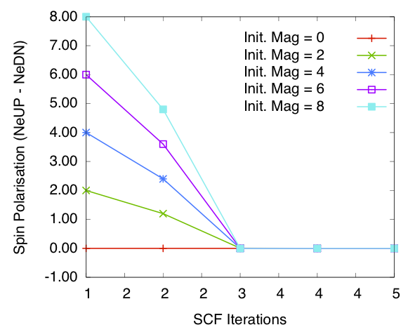
Bulk Si: spin polarisation in the cell vs self-consistency steps. Calculated using diagonalisation method and SZ PAO basis.
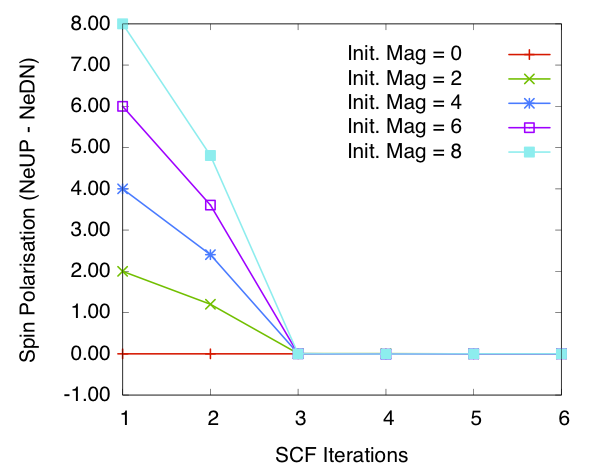
Bulk Si: spin polarisation in the cell vs self-consistency steps. Calculated using order N method and SZ PAO basis
Figures 1 and 2 show the total spin polarisation in the simulation cell for bulk silicon during the self-consistency iteration step for a spin relaxation calculation using diagonalisation and order \(N\) methods. In both cases spin polarisation converges to 0.0, confirming our expectations.
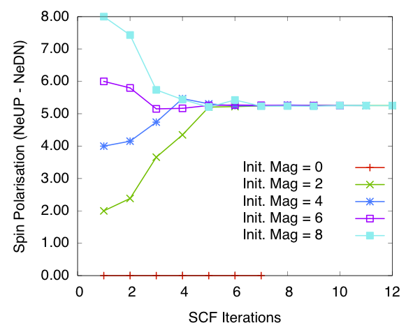
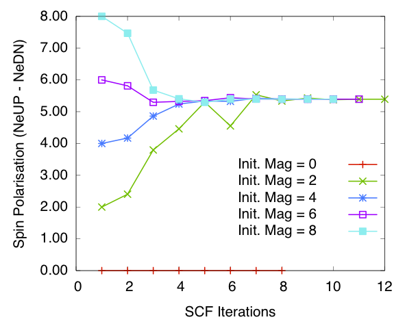
Bulk Fe: spin polarisation in the cell vs self-consistency steps. Calculated using diagonalisation method and SZ PAO basis
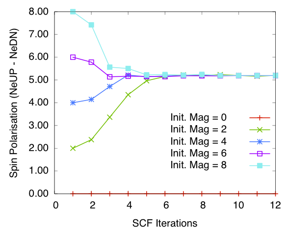
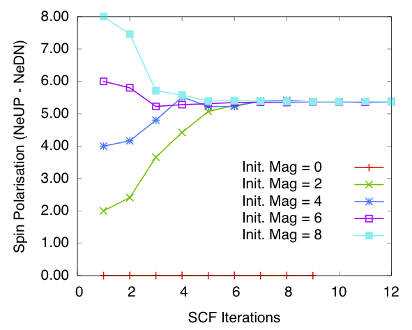
Bulk Fe: spin polarisation in the cell vs self-consistency steps. Calculated using order N method and SZ PAO basis
Figures 3 and 4 show the total spin polarisation in the simulation cell for bulk iron during the self-consistency iteration steps for a spin relaxation calculation. Both diagonalisation and order \(N\) methods are used. As we can see if the calculation starts of with 0.0 magnetisation (i.e. populations in each spin channels equal) then the magnetisation stays 0.0 through-out the self-consistency steps. This corresponds to one of the stable magnetisation states of bulk iron. Once we break the symmetry the calculations converges to a total spin polarisation of around 5.2 per cell (see the table below for more details). This corresponds to spin polarisation of 2.6 per atom, which is higher than the experimental values of 2.12. However this is expected as LDA is known to over estimate spin polarisations and we have used minimum basis set. When compared with calculations done with other codes (see below) this value is reasonable.
Bulk Fe: spin polarisation in the cell vs self-consistency steps. Calculated using diagonalisation method and blip basis
Bulk Fe: spin polarisation in the cell vs self-consistency steps. Calculated using diagonalisation method and blip basis
I have also tested calculations using the Conquest blip (B-spline) basis set, with the same number of support functions as the PAO base. At each energy minimisation step the blip basis coefficients are also optimised. The results on convergence of spin polarisation are presented in figures spinpolarisationvsiterationFeDiagblip and spinpolarisationvsiterationFeONblip. They are comparable to the PAO calculations.
The final spin polarisations per atom calculated using different methods for bulk iron with non-zero initial magnetisation is given in the following table
| Method/Code | init. mag = 2.0 | 4.0 | 6.0 | 8.0 |
|---|---|---|---|---|
| Diagonalisation, LDA, SZ (PAO) | 2.62636 | 2.62636 | 2.62662 | 2.62637 |
| Diagonalisation, LDA, Blips | 2.69637 | 2.69699 | 2.69683 | 2.69670 |
| Order \(N\), LDA, SZ (PAO) | 2.59853 | 2.59892 | 2.59795 | 2.59901 |
| Order \(N\), LDA, Blips | 2.68764 | 2.68748 | 2.68711 | 2.68829 |
Siesta, LDA, Blips | – | – | – | 2.62397 |
Note that for Siesta calculation, the same pseudopotential and
PAO SZ basis set, integration grid (\(36 \times 36 \times 36\)) and
the same Fermi smearing temperature of 300K were used.
3 Implementing van der Waals Energy Correction
The aim for the second part of this dCSE project is to implement the
ab initio van der Waals energy correction term to density functional
calculations described by Dion et al.[3] in
Conquest. The energy correction term provides a
excange-correlation functional which includes long-range
correlations essencial for modelling van der Waals interactions.
The new functional takes the form \begin{equation*} E_{\text{vdW}} = E_{\text{x}}^{\text{revPBE}} + E_{\text{c}}^{\text{PW92}} + E_{\text{c}}^{\text{nl}} \end{equation*} so that the functional takes the exchange term from a GGA functional and the correlation term from a LDA functional together with contribution from a non-local functional.
The non-local functional is given as \begin{equation} E_{\text{c}}^{\text{nl}} = \frac{1}{2} \iint \D^3\vec{r}_1\D^3\vec{r}_2\, \rho(\vec{r}_1) \rho(\vec{r}_2) \phi(q_1, q_2, r_{12}) \label{eq:Enl} \end{equation} where \(r_{12} = \norm{\vec{r}_1 - \vec{r}_2}\), \(q_i = q_0(\vec{r}_i)\), and \(q_0(\vec{r})\) is a function of \(\vec{r}\) that is dependent on charge density \(\rho(\vec{r})\) and its gradient. Its form is given by equations (11) and (12) in Dion's paper[3]. The form of the non-local functional kernel \(\phi(q_1, q_2, r_{12}) = \phi(d_1, d_2)\), where \(d_i = q_ir_{12}\) is given by equations (14) to (16) in Dion's paper.
It would be impractical to try to evaluate equation \eqref{eq:Enl} directly due to the double integral on real-space coordinates. Even for a modest grid of \(64 \times 64 \times 64\) in the simulation cell, this corresponds to \(64^6 = 68719476736\) number of evaluation of \(\phi\) and products with the two densities to evaluate the integral.
Approximations must be applied.
3.1 Overview of Approach
Roman-Perez et al.[15] proposed an efficient approximation to equation \eqref{eq:Enl}, by interpolating the non-local kernel \(\phi(q_1, q_2, r_{12})\) on a logarithmic grid of the \(q_0(\vec{r})\) values: \begin{equation*} \phi(q_1, q_2, r_{12} \approx \sum_{\alpha\beta} \phi(q_\alpha, q_\beta, r_{12}) p_\alpha(q_1) p_\beta(q_2) \equiv \sum_{\alpha\beta} \phi_{\alpha\beta}(r_{12}) p_\alpha(q_1) p_\beta(q_2) \end{equation*} where \(q_\alpha\) are points on the logarithmic grid, and \(p_{\alpha}(q_1)\) are a set of cubic spline interpolations of the delta functions \(\delta(q_1 - q_\alpha)\) whose values at the grid points are \(\delta_\beta = \delta_{\alpha,\beta}\).
By approximating the kernel this way, the dependence on \(q_1\) and \(q_2\) are now separated, and hence equation \eqref{eq:Enl} can be approximated as \begin{equation*} E_{\text{c}}^{\text{nl}} \approx \frac{1}{2} \iint \D^3\vec{r}_1\D^3\vec{r}_2\, \sum_{\alpha\beta} \theta_{\alpha}(\vec{r}_1) \phi_{\alpha\beta}(r_{12}) \theta_{\beta}(\vec{r}_2) \end{equation*} where \(\theta_{\alpha}(\vec{r}_i) = \rho(\vec{r}_i) p_\alpha(q_i)\). The equation above now contains a convolution and hence when working in the Fourier transform space we have \begin{equation} E_{\text{c}}^{\text{nl}} = \frac{1}{2} \int\D^3\vec{k}\, \tilde{\theta}^*_{\alpha}(\vec{k}) \tilde{\theta}_{\beta}(\vec{k}) \tilde{\phi}_{\alpha\beta}(k) \label{eq:EnlFFT} \end{equation} The calculation thus becomes manageable.
\(\phi_{\alpha\beta}(r_{12})\) is a radial function, and hence a
radial FFT subroutine needs to be implemented in Conquest in
order to obtain \(\tilde{\phi}_{\alpha\beta}(k)\). The
\(\theta_\alpha(\vec{r})\) functions are ordinary functions on the 3D
real grid, and hence can be Fourier transformed by the existing
FFT algorithms implemented in Conquest.
3.2 Grids
There are several different types of grids used for the implementation.
- First of all there is the
Conquest's own integration/FFT grid, distributed among the processors, on which the values of \(\theta_\alpha(\vec{r})\) and their Fourier transforms will be stored. - There is the grid for the \(q\) values, and upon which each value of \(\phi_{\alpha\beta}(r)\) (for fixed \(r\)) and polynomials \(p_{\alpha}\) are defined. These are logarithmic grids, and following advice from the paper[15], I have defined 30 grid points for this grid. And this grid is local to each processor.
- Further more, there is the radial grid, upon which the values of \(\phi_{\alpha\beta}(r)\) is calculated for fixed \(\alpha\) and \(\beta\). Since the radial grid is one dimensional (and hence relatively small) and Fourier transforms will be done on this grid, it is sensible to make this grid local to each processor as well. For the moment I have fixed the grid size to 1024. This is dense enough for most calculations, but still tiny when compared with the 3D real-space grid.
The final integration for calculating the non-local energy
\(E_{\text{c}}^{\text{nl}}\) is done on the Conquest
integration/FFT grid. However if we simply use the radial Fourier
transforms of \(\phi_{\alpha\beta}(r_{12})\) calculated on the radial
grid, we will cause errors due to inconsistencies of the two
different grids. Hence the \(\tilde{\phi}_{\alpha\beta}(k)\)
calculated will be interpolated results from the values
calculated on the radial grid.
3.3 Implementation of Radial FFT
To calculate the Fourier transforms of \(q(r)\) defined on the radial
grid, I have to implement a version of radial FFT in Conquest.
We note that for any radial function \(f(\vec{r}) = f(r)\) the Fourier transform may be written in spherical polar coordinates with the \(z\)-axis defined to coincide with vector \(\vec{k}\), as: \begin{equation*} F(\vec{k}) = 2\pi \int_0^\infty \D{r}\, \int_0^\pi \D\theta\, r^2 \sin(\theta) e^{-i2\pi k r \cos(\theta)} f(r) \end{equation*} where \(k = \norm{\vec{k}}\). The \(\theta\) integral may be evaluated to give \begin{equation*} \int_0^\pi \D\theta \sin(\theta) e^{-i2\pi k r \cos(\theta)} = \left[ e^{-i2\pi k r \cos(\theta)} \right]^\pi_0 \frac{1}{i2\pi k r} = \frac{2\sin(2\pi k r)}{2\pi k r} \end{equation*} Therefore: \begin{equation} F(\vec{k}) = F(k) = \int_0^\infty \D{r}\, \frac{2\sin(2\pi k r)}{2\pi k} r f(r) \label{eq:contFFT} \end{equation} In other words the Fourier transform of a radial function is also radial.
Now we need to discretise equation \eqref{eq:contFFT}. If the real space radial grid goes from 0 to \(r_{\text{max}}\) with \(N\) data points then \begin{equation*} F_j \approx dr \sum_{i=0}^{N-1} \frac{2 \sin(2\pi idr jdk)}{jdk} idr f_i \end{equation*} where \(i = 0, N-1\) indices the real space radial grid and \(j = 0, N-1\) indices the reciprocal grid. \(dr = r_{\text{max}} / N\), and \(dk\) is given in terms of the Nyquist critical frequency associated to the chosen real space grid. The critical frequency is given[13] as \(f_c = \frac{1}{2dr}\). This is the maximum possible \(k\) value beyond which point any non-zero F(k) values will be folded back and causing aliasing. Hence it is the usual practice to set the maximum \(k\) value on the discrete FFT radial grid to be \(f_c\). So going from 0 to \(f_c\) with \(N\) points, \(dk = \frac{1}{2Ndr}\). Therefore substitute the value of \(dk\) into the above equation, we obtain \begin{equation*} F_j \approx \frac{dr}{jdk} \sum_{i=0}^{N-1} 2 \sin(2\pi ij/N) idr f_i \end{equation*} Define \(g_i \equiv 2idrf_i\) we thus have \begin{equation} F_j \approx \frac{dr}{jdk} \sum_{i=0}^{N-1} \sin(2\pi ij/N) g_i \label{eq:discFFT} \end{equation} where unless \(f_i \sim \frac{1}{idr^n}\) for integer \(n > 1\), \(g_i = 0\) at \(i = 0\). Hence baring the special case for \(f_i\) (which will be outside the range of functions we will need to consider) the sum in equation \eqref{eq:discFFT} is just a standard discrete sin transform[13].
There is a logarithmic singularity at \(k = 0\) due to the
\(\frac{1}{k}\) factor in equation \eqref{eq:contFFT}, and therefore
the \(k = 0\) point is treated separately. If \(k = 0\) then \(\lim_{k
\to 0} \sin(2\pi k r){k} = 2\pi r\). Hence after discretisation
\begin{equation*}
F_0 \approx dr \sum_{i=0}^{N-1} 4\pi (idr)^2 f_i
\end{equation*}
Thus the algorithm for radial FFT implemented in Conquest is as
follows
subroutine radfft(func, func_out, n_r, dr)
  dk = half / real(dr * n_r, double)
  ! set the real data to 2 * r * func(r)
  do ir = 1, n_r
    rr = (ir - 1) * dr
    data(ir) = two * rr * func(ir)
  end do
  ! do sin FT
  call sinft(data, n_r) ! from Numerical Recipes
  ! leave the k = 0 point aside, this is treated separately
  do ik = 2, n_r, 1
    kk = (ik - 1) * dk
    func_out(ik) = data(ik) / kk
  end do
  ! doing the k = 0 point
  ! the limit (k -> 0) of 2 * r * sin(2*pi*k*r) / k is 4*pi*r**2
  func_out(1) = zero
  do ir = 1, n_r
    rr = (ir - 1) * dr
    func_out(1) = func_out(1) + (four * pi * rr**2 * func(ir))
  end do
  ! scale func_out by to give approximation to non-discrete form
  func_out = dr * func_out
end subroutine
It is important to note that radfft calculates the approximation
of the continuous radial Fourier transform, unlike a standard FFT
subroutine, which calculates the discrete Fourier transform of a
given set of data points.
The grid size must be of integer powers of two.
The subroutine has been tested against and shows good agreement to the analytical results calculated from Mathematica on various gaussian functions.
3.4 Implementation of van der Waal Energy Correction
The non local correlation energy \(E_{\text{c}}^{\text{nl}}\) given in equation \eqref{eq:EnlFFT} are calculated in Conquest as follows.
subroutine vdWXC_nl_energy(rho, E_vdW_nl)
1. From the Conquest integration/FFT mesh get mesh spacing
2. From FFT mesh spacing, calculate Nyquist critical frequency and
   hence kcut and dk
3. Set up q-mesh (logarithmic)
4. Calculate phi(r, q1, q2), and its Fourier transform for each
   points q1, q2 on the q-mesh and r (and k) on the radial mesh as
   well as the second derivatives and store the interpolation table
   in file vdW_kernel.tab
5. Calculate gradient of rho (density) and store in grho
6. Calculate polynomials p(q1) as a function of rho and grho
   6.1 Calculate the value of q from rho and grho
   6.2 Interpolate p(q1) from given q for every q1 on q-mesh
7. From p(q1) and rho calculate theta(vec_r,q1)
8. FFT theta(vec_r,q1) on Conquest FFT grid for every q1 on q-mesh
9. Loop over FFT grid points
     Calculate mag_k = sqrt(sum(vec_k**2)) for a given vec_k on grid point
     if (mag_k < kcut) then
       Interpolate from the vdW_kernel table to get phi(k,q1,q2)
       calculate the complex matrix multiplication and dot product on q-mesh
         phi(k,q1,q2) * theta(vec_k,q1) theta(vec_k,q2)
       Accumulate into E_vdW_nl (for non-local energy)
     end if
   end Loop
10. Gather and reduce values of E_vdW_nl distributed among the processors
end subroutine vdWXC_nl_energy
The over all van der Waals exchange-correlation energy is the calculated as a sum of \(E_{\text{c}}^{\text{nl}}\) (calculated above), the exchange part of revPBE functional and the correlation part of PW92 function.
When used in actual applications, Conquest first runs a
self-consistent calculation with either one of the LDA or GGA
functionals, and after it reached self-consistency the van der
Waals exchange-correlation energy is then calculated using the
self-consistent density. The van der Waal energy correction is then
calculated by subtracting the original LDA/GGA exchange-correlation
energy from the calculated value.
3.5 Test Results
Test runs have been performed on a system of two benzene rings,
stacked one directly on top of the other along the concentric
axis. Interaction energies of the benzene rings can be calculated
by taking the difference in total energy between the two ring
system and 2 times a single benzene system. The van der Waals
correction to interaction energies are calculated by first
calculating interaction energies calculated using either LDA or GGA
functionals, and then subtract this from the interaction energies
calculated with van der Waals energy correction turned
on4. The calculated results are then compared with results
calculated from Siesta, which has implemented the same van der
Waals functional. It has to be noted however that the comparison can
not be exactly due to the fact that in Siesta the van der Waals
functional is self-consistent and hence unlike in Conquest
calculation the results are calculated using van der Waals function
(potential) through out.
The simulation cell (for both Conquest and Siesta calculations)
was set to be cubic, with lattice parameter set to 20.0 Ang on all
sides. The number of grid points are set to be \(128 \times 128
\times 128\). For Conquest calculations pseudopotential and basis
sets are generated by either LDA or GGA functionals (which ever is
under comparison), for Siesta calculations, the LDA and GGA
results are calculated using identical pseudopotential and basis
sets as that used by Conquest, however the van der Waals used
pseudopotentials and basis sets generated by van der Waals
functional.
System of two benzene molecules stacked one directly on top of the other along the concentric axis.
System of two benzene molecules stacked one directly on top of the other along the concentric axis.
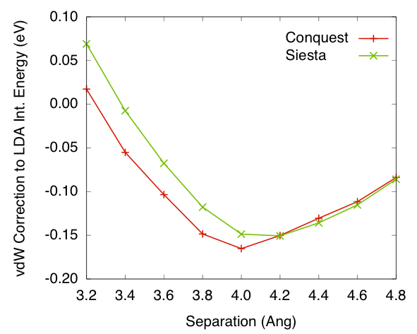
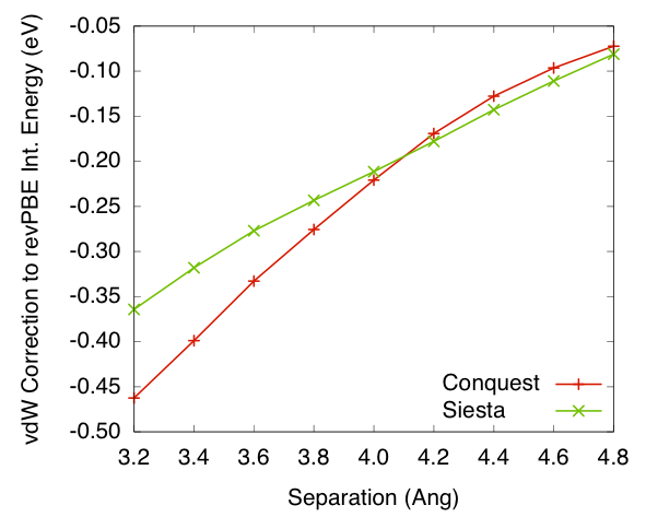
Figures 5 and
6 shows the van
der Waals correction to interaction energies for system calculated
either using PW92 LDA or revPBE GGA. The values are plotted against
separation distances between the two benzene rings. The results
show reasonable agreement between the Conquest implementation and
Siesta implementation, bare in mind that the Siesta calculation
is self-consistent while Conquest is not.
The table below shows the total execution time taken for the van der Waals correction implementation and its percentage in relation to the total program run time. The test calculation is done on two benzene rings using revPBE functional with van der Waals correction with an integration grid size of \(128 \times 128 \times 128\). It took 6 SCF steps for the calculation to converge
| Number of Nodes | Total run time (s) | vdW time (s) | Ratio |
|---|---|---|---|
| 1 | 339.730000 | 156.125000 | 0.459000 |
| 2 | 217.320000 | 116.082030 | 0.534000 |
| 4 | 131.870000 | 93.398440 | 0.708000 |
It can be seen that the van der Waals correction subroutines does cost a significant portion of the total run time. There is also an indication that it becomes less efficient compared to the rest of the code when number of computation nodes increases.
The code generates the interpolations of the non-local kernels when it first runs. For the subsequent runs the results are simply read from the table at start up. The following shows the times taken if the table has been pre-generated
| Number of Nodes | Total run time (s) | vdW time (s) | Ratio |
|---|---|---|---|
| 1 | 309.060000 | 133.914060 | 0.433000 |
| 2 | 196.290000 | 95.933590 | 0.488000 |
| 4 | 113.660000 | 76.636720 | 0.674000 |
Slight improvements on performance can be observed.
The long processing time can be expected, due to the nature of the algorithm. For the calculation of the non-local correlation energy \(E_{nl}\), we have to do a matrix product and a dot product on the \(q\)-mesh, for every integration point on the 3D FFT mesh. This amounts to \(30^2 = 900\) times the work-load compared to a typical electron number calculation or an inner product between the residuals.
This can be confirmed by following table, which shows break downs on the major parts of the van der Waals code:
| Area | Time/Ratio (s) (1 node) | 2 nodes | 4 nodes |
|---|---|---|---|
| Generate \(\phi\) table | 19.390630 (0.124) | 18.445310 (0.158) | 18.195310 (0.194) |
| build \(\grad{\rho}\) | 2.613280 (0.016) | 2.832030 (0.024) | 2.156250 (0.023) |
| build \(\theta\) | 2.253910 (0.014) | 1.066410 (0.009) | 0.625000 (0.006) |
| FFT \(\theta\) | 19.429690 (0.124) | 21.257810 (0.183) | 24.472660 (0.262) |
| Integrate \(E_{nl}\) | 78.988280 (0.505) | 49.218750 (0.423) | 25.640630 (0.274) |
This clear shows that for small number of nodes the \(\vec{k}\) space integration is the most expensive part of the implementation. However as the number of nodes increase FFT quickly becomes the new bottle neck. This also also explains the apparently poor scaling displayed by the code. Because the implementation requires 30 FFTs to be done the communication inefficiencies of the FFT routines quickly becomes a significant factor. Note that the poor scaling in the \(\phi\) table generation part is mainly due to only one node is doing all the IO during the writing to file phase, and this process is expected to be slow and non-scaling.
If the non-local kernel table has been pre-generated, then we can see clearly that significant amount of work can be avoided.
| Area | Time/Ratio (s), 1 node | 2 nodes | 4 nodes |
|---|---|---|---|
| Generate \(\phi\) table | 0.187500 (0.001) | 0.187500 (0.001) | 0.203130 (0.002) |
| build \(\grad{\rho}\) | 2.851560 (0.021) | 2.175780 (0.022) | 2.847660 (0.037) |
| build \(\theta\) | 1.878910 (0.014) | 1.062500 (0.011) | 0.507810 (0.006) |
| FFT \(\theta\) | 18.902340 (0.141) | 18.785160 (0.195) | 24.929690 (0.325) |
| Integrate \(E_{nl}\) | 76.058590 (0.567) | 50.558590 (0.527) | 25.847660 (0.337) |
The table below shows memory usage by the implementation:
| Calc Type | Maximum RSS (MB) per node, 1 node | 2 nodes | 4 nodes |
|---|---|---|---|
| vdW without table | 2021.910156 | 1053.257812 | 549.960938 |
| vdW with table | 2021.851562 | 1053.210938 | 547.882812 |
| Vanilla (no vdW) | 1017.695312 | 545.023438 | 276.968750 |
The van der Waals implementation uses twice the amount of memory as
the original code. My initial version of the implementation uses
even more memory, due to the fact that original Conquest
implementations of exchange-correlation functionals takes in the
grid data arrays as input and output. This required a number of
temporary storages for passing grid data from one subroutine to
another. To reduce memory I changed the implementation of these
functional act point-wise on the grid data. While this introduced
inefficiency as the exchange-correlation functional subroutines
have to be called at every grid point, it reduced memory usage
significantly (by about factor of three). However even after this
memory usage is still large.
This high memory usage is caused by the fact that there are 30 \(\theta\) functions—one for every point on the \(q\)-mesh, all of which are data points on the real/FFT grid—we need to store at the same time. We cannot do this one by one because a pair of the functions are required at any one time in the integral for calculating \(E^{\text{nl}}_{\text{c}}\), and we have to go through all permutations of the pairings. One could in theory recalculate the \(\theta\) functions at every integration accumulation step, but that will lead to a lot of unnecessary re-evaluation of the \(\theta\) functions and their Fourier transforms. Considering FFT becomes the bottle neck for more processors I believe doing this would be unwise.
4 Conclusion and Future Work
Both spin polarisation and van der Waals functional have been
successfully implemented and test calculations gives expected
results. For spin relaxation calculations the new energy minimisation
scheme and Pulay mixing scheme for self-consistency has been tested
and demonstrated to be working. The data structure of Conquest now
handles spin polarisation naturally, and efforts has been made to
make the existing subroutines to handle both spin non-polarised and
polarised calculations. This helps to make future developments in
Conquest easier, the developer do not have to develop separate
versions codes for spin non-polarised and polarised calculations.
Four out of the six exchange-correlation functionals implemented in
Conquest has been extended to work with spin polarised
calculations. Future work remains for converting the rest. While the
spin polarised version of non-self-consistent forces has been
implemented for a LDA functional, the derivation of equations for
the GGA functionals are left for future work due to its
complexity. Protective warning messages and default behaviours have
been added in the code to prevent the user from making wrong choice
of functionals and force settings when running a spin polarised
calculation.
Memory usage is a big concern with the implementation of van der
Waals functions. As it is shown in test calculations, the memory
usage with van der Waals correction turned on is almost twice of
standard calculations. The fundamental reason for high memory usage
seems to be due to the functional form used to approximate the
functional. This same problem has been observed in
Siesta. Never-the-less this approximation made a functional
previously impractical to use (due to its double integration and
non-local nature) practical.
Due to the large number of grid integrations one needs to perform,
van der Waals functional is relatively expensive computationally, in
our test calculations it has the equivalent cost of roughly 6 energy
minimisation operations. While integration on grid shows good
scalability with number of nodes, the over all scalability of the
code is hampered by the extensive use of FFT. For calculation of
large systems, a more efficient FFT engine would benefit. At the
moment Conquest uses its own FFT implementation, and future work
could be done to allow Conquest to use standard external FFT
libraries optimised for HCP platforms.
It is also possible in the future to extend the van der Waals implementation for self-consistent calculations. This involves finding the potential by calculating the derivatives of the functional with respect to density.
At the moment most of the grid settings for the logarithmic and radial grid used by van der Waals functional are defined as parameters in the code. While those seldom needs to be changed, in the future it would be beneficial to include them as part of the input changeable by the user.
The spin implementations has already been submitted to Conquest
code repository and implementation of van der Waals functional will
be submitted shortly. The beta release of Conquest can be obtained
from http://www.order-n.org/.
5 Acknowledgement
This project was funded under the HECToR Distributed Computational Science and Engineering (CSE) Service operated by NAG Ltd. HECToR—A Research Councils UK High End Computing Service—is the UK’s national supercomputing service, managed by EPSRC on behalf of the participating Research Councils. Its mission is to support capability science and engineering in UK academia. The HECToR supercomputers are managed by UoE HPCx Ltd and the CSE Support Service is provided by NAG Ltd. http://www.hector.ac.uk
Footnotes:
1 This means the spins of the electrons in the system under study are aligned, so spin states can be either "up" or "down".
2 In the case of spin non-polarised calculation the Fermi energies of the spin channels happen to be the same due to symmetry of the two channels.
3 The inner product between two residual functions \(R_n\) and \(R_m\) is defined by \(\inner{R_n}{R_m} \equiv \int\D^3\vec{r}\, R_n(\vec{r}) R_m{\vec{r}}\); and the norm of \(R_n\) is simply \(\norm{R_n} = \sqrt{\inner{R_n}{R_n}}\).
4 The same LDA or GGA functional is used to compute the self-consistent density prior the van der Waals correction step.
References
| [1] | D. R. Bowler. Linear-scaling density matrix minimisation and electron number conservation. Technical report, University College London, 2005. |
| [2] | D. R. Bowler, I. J. Bush, and M. J. Gillan. Practical methods for ab initio calculations on thousands of atoms. Int. J. Quantum Chem., 77(5):831-842, 2000. [DOI | http ] |
| [3] | M. Dion, H. Rydberg, E. Schroder, D. C. Langreth, and B. I. Lundqvist. Van der waals density functional for general geometries. Phys. Rev. Lett., 92(24):246401, 2004. [http ] |
| [4] | S. Goedecker, M. Teter, and J. Hutter. Separable dual-space gaussian pseudopotentials. Phys. Rev. B, 54(3):1703-1710, Jul 1996. [DOI | http ] |
| [5] | B. Hammer, L. B. Hansen, and J. K. Nørskov. Improved adsorption energetics within density-functional theory using revised perdew-burke-ernzerhof functionals. Phys. Rev. B, 59:7413-7421, Mar 1999. [DOI | http ] |
| [6] | G. Kresse and J. Furthmüller. Efficiency of ab-initio total energy calculations for metals and semiconductors using a plane-wave basis set. Computational Materials Science, 6(1):15-50, July 1996. [http ] |
| [7] | R. M. Martin. Electronic Structure: Basic Theory and Practical Methods. Cambridge University Press, 2004. |
| [8] | A. H. R. Palser and D. E. Manolopoulos. Canonical purification of the density matrix in electronic-structure theory. Phys. Rev. B, 58(19):12704-12711, Nov 1998. [DOI | http ] |
| [9] | J. P. Perdew, K. Burke, and M. Ernzerhof. Generalized gradient approximation made simple. Phys. Rev. Lett., 77(18):3865-3868, Oct 1996. [DOI ] |
| [10] | J. P. Perdew, K. Burke, and M. Ernzerhof. Perdew, burke, and ernzerhof reply:. Phys. Rev. Lett., 80(4):891, Jan 1998. [DOI ] |
| [11] | J. P. Perdew and Y. Wang. Accurate and simple analytic representation of the electron-gas correlation-energy. Phys. Rev. B, 45(23):13244-13249, June 1992. |
| [12] | J. P. Perdew and A. Zunger. Self-interaction correction to density-functional approximations for many-electron systems. Phys. Rev. B, 23(10):5048-5079, 1981. |
| [13] | W. H. Press, S. A. Teukolsky, W. T. Vetterling, and B. P. Flannery. Numerical Recipes in Fortran 77: The Art of Scientific Computing, volume Volume 1 of Fortran Numerical Recipes. Cambridge University Press, second edition edition, 2001. |
| [14] | P. Pulay. Convergence acceleration of iterative sequences. the case of scf iteration. Chem. Phys. Lett., 73(2):393-398, 1980. [DOI | http ] |
| [15] | G. Román-Pérez and J. M. Soler. Efficient implementation of a van der waals density functional: Application to double-wall carbon nanotubes. Phys. Rev. Lett., 103(9):096102, Aug. 2009. [http ] |
| [16] | L. Tong. Metal conquest. Technical report, UCL and NAG, Mar. 2011. [http ] |
| [17] | A. S. Torralba, D. R. Bowler, T. Miyazaki, and M. J. Gillan. Non-self-consistent density-functional theory exchange-correlation forces for gga functionals. J. Chem. Theory Comput., 5(6):1499-1505, June 2009. [DOI ] |
| [18] | I. Wolfram Research. Mathematica edition: Version 7.0, 2008. |
This file was generated by bibtex2html 1.96.