1 Introduction

As computing hardware has become more powerful, computational science has largely kept pace with the available resources, exploring larger; more complex and often more physically accurate systems. An area of Physics and Chemistry where this is particularly true is in DFT where calculations have always pushed the largest supercomputers to their limit; from the vector systems of the 80s, through the bespoke and diverse distributed memory landscape of the 90s to the current situation of hybrid shared and distributed memory, highly parallel supercomputers with relatively homogeneous architecture. DFT calculations have scaled from 8 atom silicon unit-cell systems, up to thousands of atoms in bulk metallic systems and tens of thousands of atoms in organic molecules.

These calculations are exploring single points in configuration space, however, and in order to have truly converged, physical results one must minimise not only the energy of the electronic structure with fixed ions, but also of ionic position. Computationally this is a much larger task; while the division of labour between the geometry and electronic calculations burdens the electronic minimisation more heavily, each iteration of a geometry minimisation must perform a single-point electronic minimisation in order to find the forces with which to minimise the structural energy.

As it stands, CASTEP and ONETEP share BFGS geometry optimiser code which was written at a time when it was not feasible to study systems larger than 1000 atoms with DFT. BFGS is a quasi-Newton method which builds up an approximation to the Hessian with rank-2 updates in ionic position and energy-gradient. Since the Hessian is a “degrees of freedom squared” object, the storage required in a geometry optimisation is maximally of the order(6 + 3N)². This includes the 3 degrees of freedom (DoF) of each ion in 3-dimensional space and the 6 DoF (excluding rotations, which ought to be energy invariant) in the cell space, bearing in mind that DoF are reduced by constraints and that ONETEP cannot currently do variable cell calculations.

Large systems will quickly consume all of the memory on a node, since the quadratically scaling Hessian is duplicated on every MPI image and not distributed. The problem is compounded by the fact that the Hessian needs to be frequently re-initialised to obtain good convergence characteristics and the process of producing an initialisation, as outlined by Pfrommer et al, is implemented with 6 further Hessian-sized matrices.

The original goals of the dCSE project were as follows:

1. Familiarisation with existing BFGS algorithm and implementation.
2. Optimisation of existing BFGS code in CASTEP (e.g. more efficient use of BLAS).
3. Implementation of basic L-BFGS algorithm in CASTEP.
4. Implementation of L-BFGS within SVD code in CASTEP (inverse Hessian).
5. Implementation of new algorithms into ONETEP.
6. Investigate performance (time and memory) of new algorithm on large benchmarks.
7. Finish documentation, integrate into main codebase and write final report.

2 BFGS Method

The Broyden, Goldfarb, Fletcher and Shanno (BFGS) method is an approximation to Newton’s method for solving non-linear optimisation problems. It builds on earlier quasi-Newton methods such as the Davidon, Fletcher, Powell (DFP) method, but provides superior convergence characteristics [3]. Furthermore, when compared to steepest-descents and conjugate-gradients (CG) approaches, quasi-Newton methods often present a more direct path to the stationary point, as a better model of the functional geometry has been built through the knowledge and application of the curvature information [5]. Quasi-Newton methods have a clear disadvantage compared with CG however, when it comes to memory use, since BFGS builds up a Hessian which is O(N²).

2.1 Newton’s Method

A twice-differentiable scalar field f can be Taylor expanded about a point x,

(1)

where is the Jacobian and is the Hessian.

Then, if the differential of this function with respect to△x is set to zero, the local stationary point of this approximation may be found, with respect to the expansion point,

(2)

This process can be iterated in order that stationary points of f may be found, provided that the function is Taylor expanded close enough to the minimum that it is well approximated,

(3)

In order to satisfy the Wolfe conditions, the step size must be scaled by α,

(4)

and the process is iterated until numerical convergence.

2.2 Quasi-Newton Methods

In the vicinity of the stationary point, the Newton method provides good convergence properties and level of accuracy. Its drawback is primarily that it requires the calculation of a full Hessian, which is computationally expensive and needs N² memory. An alternative is to build up an approximation to the Hessian from low-rank updates at each iteration, with the aim of reproducing some important properties of the Hessian, which eases the first problem. This is known as a Quasi-Newton method, of which there are many variations on this theme, however, decades of numerical experience has shown some updates to the Hessian to have superior convergence characteristics.

2.2.1 BFGS

The most important property which the Hessian must imitate is that it obeys the secant equation, or that the matrix can be used to transform between a change in position and a change in gradient,

(5)

where s_n and y_n are the change in position and gradient vectors, respectively.

One of the most successful and widely used update formulae is BFGS, due to its stability, good convergence with an inexact line-search and that it maintains the symmetry and positive-definiteness of the Hessian approximation.

The update formula is given as:

(6)

where ρ_k = . It can be seen from eq.(6) that the BFGS formula updates the inverse of the Hessian matrix, ^-1 (which will be referred to as from hereon in). This is especially useful when the scheme is used in anger, as at each iteration, the Hessian is then used to find a search direction to minimise along, and hence find the point at which to perform the next iteration. This is performed in the following way:

(7)

so compared with a scheme such as DFP (Davidon-Fletcher-Powell), which updates the Hessian and subsequently requires its inversion, this latter step might be avoided by updating the inverse Hessian instead. It is worth noting that the Sherman-Morrison-Woodbury (SMW) formula states that the inverse to a rank-n update to a matrix can equivalently be calculated as a rank-n update to the inverse of the initial matrix

(8)

This can be applied to either BFGS or DFP, in order to update the Hessian and inverse Hessian matrices instead, respectively.

2.3 Line Search

Because the quasi-Newton model is not necessarily accurate, especially where a small number of updates have been used, or when in the anharmonic limit, a line search is often used to give a value for α (see eq. 4 on page §). Specifically, this means that the quasi-Newton, parabolic model is used to construct a search direction and the exact function is minimised along this line. It is often impractical to perform a precise line-search, since this will only mean more minimisation cycles. For efficiency, the precision of the line search must be balanced against the number of quasi-Newton steps so as to reduce function (force) evaluations.

(9)

2.4 Wolfe Conditions

Performing a line search in practice is a compromise; the idea is to find the minimum of the objective function along the search direction. However in order to do this well, the correct step-length, α, must be calculated. It follows that several points along the search direction must be explored and for each point a function evaluation computed. The Wolfe conditions are a pair of conditions on the step-length which ensure not that the global minimum has been found, but whether an arbitrarily defined reduction has been found in the function for a particular α (and that α is not small, so that the process makes reasonable progress). The first Wolfe condition, that sufficient decrease is seen in the objective function is:

(10)

and the second, that a large enough step-size is chosen is:

(11)

The coefficient scalars w₁ and w₂ are chosen arbitrarily, but through experience, the first should be small and the second, “a bit” less than 1 (0.8 perhaps). In the CASTEP line-search, the second condition is not necessary, as a backtracking line-search is used, which starts from a non-negligible fixed value.

3 Limited Memory BFGS

In order to improve the memory scaling of BFGS (and quasi-Newton updates, in general), the structure of the update needs to be examined carefully. It has been shown [2] that the recursive representation eq.(6) is equivalent to:

(12)

where:

(13)

₀ is the initial inverse Hessian,

(14)

(15)

(16)

s_n and y_n are the n^th position and gradient update vectors, respectively. While this is a more complicated representation than that in eq.(6), the advantage is that since the only operation we will ever perform with the inverse Hessian once we have it is a multiplication by a vector, we can store the matrices of position and gradient updates, only.

In reality much of the computation at the n^th step is duplicated from the previous step, so R_n^-1 is stored and updated in the fashion suggested by eq.(14) at each step. Then through careful manipulation, W_n is never stored, and we store only matrices of size m² (where m is the number of update pairs stored or BFGS iterations), R_n and (T_n = D_n + Y _n^T₀Y _n); and matrices of the size m × n, S_n and Y _n.

While in BFGS the Hessian can be applied to give a search direction by multiplication by a force vector (see eq. 7), in LBFGS, the Hessian is never computed (or stored). For this reason an approach has to be worked out to perform the operation without ever multiplying out the expression, so as to keep the process linear scaling in memory. That algorithm is outlined as follows with the name of the corresponding BLAS call required, where v is the vector to be multiplied by the inverse Hessian and p is the resultant vector:

Function f : ℝn → ℝn, pnv
p	= 0v		DSBMV
w1:m	= Y nTp		DGEMV
wm+1:2m	= SnTv		DGEMV
w1:m	Rn-1Y nT 0v		DTRSM
wm+1:2m	Rn-1S nTv		DTRSM
Ξ	= Tn			(1)
Ξ	Rn-1Ξ		DTRSM
w1:m	w1:m - Ξwm+1:2m		DGEMV
p	p + SnTw 1:m		DGEMV
t	= -Y nTw m+1:2m		DGEMV
p	p + 0t		DSBMV
End Function

3.0.1 Limited History

The LBFGS approach allows for a very important distinction from BFGS, which turns out to be its most salient feature; the inverse Hessian approximation can be updated by removing a pair of updates without reconstruction. In practice, this means that the last k updates can be used for the construction and hence the reason why LBFGS can be considered a linearly scaling approach, in memory. In fact, if the number of updates is left unbounded, the amount of memory required will, possibly exceed that used in BFGS.

In order to allow a limited history length, routines to delete the oldest update pairs are required, effectively shifting of the end of the storage matrices.

There is, however, a further complication to using LBFGS in an atomic geometry optimiser:

3.0.2 Hessian Analysis

The very reason for LBFGS is to make the procedure linear in memory and as such re-initialisation or final analysis (for a restart, perhaps) cannot be performed without violating this premise. A way to extract elastic properties and phonon frequencies (at the centre of the Brillouin zone) was developed, and is detailed in the following section. In the project proposal, this was termed the SVD part of the project because a singular value decomposition was used to find a basis in the update space as part of the procedure. This was performed differently in the implementation of LBFGS and has been termed the “Hessian analysis” section, instead

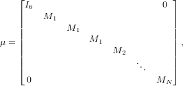
This all hinges on the inverse Hessian initialisation scheme in Pfrommer et al [6]. This works on the premise that the initial inverse Hessian is set up as follows:

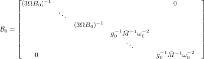(18)

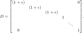
which is block-diagonal, but further to this, it is diagonal in the upper-left 9x9 quadrant and 3x3 block-diagonal in the following block. Ω is the cell volume, B₀ the bulk modulus, M the average ionic mass, ω₀^-2 the average phonon frequency at the centre of the Brillouin zone, and the matrix g₀ is the 3x3 metric tensor.

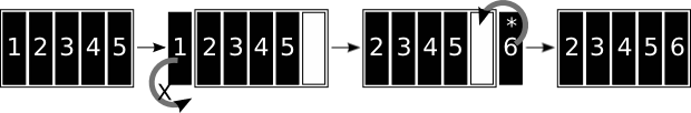
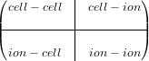
The upper-left block represents cell-cell interaction and the lower- right, ion-ion interactions; this representation does not, then model any inter-atomic blocks or acoustic modes in the cell-ion domain. Each 3x3 block on the diagonal is also symmetric, so the entire matrix can be stored as a symmetric, penta-diagonal band matrix. i.e.

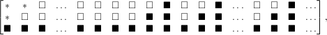(19)

where black squares represent elements of the blocks of the initial inverse Hessian, white squares are zero and * represents elements which are never accessed.

Hence, the storage requirements for the initial, inverse Hessian become linear. There is the argument that no initial inverse Hessian need ever be stored and instead only the scalars associated with its construction, and invoking a bespoke multiplication routine whenever multiplication by the inverse Hessian is required. This approach was rejected, however, since the scope for less homogeneous initialisations in the future was desirable.

Whenever a multiplication of the initial inverse Hessian by a vector was required, the BLAS routine, DGBMV can be used, however whenever a general matrix needs to be multiplied by ₀, no routine is available in BLAS or LAPACK, so one was created for the purpose. Only penta-diagonal matrices with super-diagonal bandwidth of 2 were required, so the routine retains this limitation.

In the current CASTEP code for extracting phonon modes and elastic properties, the Pfrommer paper is followed explicitly. Before the extraction begins, _n is corrected for finite strain, which enters the matrix because of how the Pfrommer process augments the force vector:

(20)

where the D matrix is defined as:

(21)

In CASTEP, this matrix is allocated in full (ndim²), before it is inverted. Because the structure of the matrix is block diagonal in the upper left quadrant and I_ndim in the remaining non-zero block, the duplicated 3x3 block, ϵ_f = (1 + ϵ) can be stored, rather than the whole matrix, inverted and multiplied by each of the 3x3 blocks along the cell-cell quadrant of , in the following fashion:

(22)

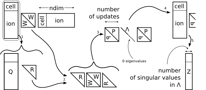
Next in the routine, to get a basis which spans the sampled subspace of the Hessian, Pfrommer proposed an SVD (singular value decomposition) of the update-space Hessian, that is all changes which have been applied to it since the initial inverse Hessian was the latest representation. This is the way the scheme is performed in CASTEP for BFGS:

(23)

where ′ is the update to the inverse Hessian, since the last initialisation of _o; V is an orthogonal matrix of the singular vectors of ′; σ is a matrix of its singular values along the diagonal and W is an orthogonal matrix of the vectors of ′ spanning its null space. As it stood, LAPACK was used to compute the N² matrix, V; while the singular values are packed into an N element vector and the right-hand vectors are never computed.

To avoid having to multiply out (12), and perform the SVD, involving at least this and a further N² objects, the structure of the decomposed LBFGS representation of ′ was examined carefully,

(24)

we know that the update matrices are not necessarily orthogonal, however a QR factorisation fixes this. The product is never multiplied out, but in principle this is what is implied at this point:

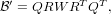(25)

now, RWR^T can be spectrally decomposed:

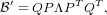(26)

where Λ is the matrix of eigenvalues and P, the orthogonal matrix of eigenvectors of the decomposition. Since Q and P are both orthogonal, it is plain that their product is also orthogonal and hence we have extracted a basis in the update space of the inverse Hessian without ever forming it explicitly. We only store the elements of QP which have a corresponding, non-zero singular value in Λ, this max(N*M) matrix will be called Z.

An important ambiguity in the Pfrommer paper is the statement that the basis, Z should be comprised of pure cell and pure ion vectors. The interpretation of this in the original CASTEP logic resulted in an SVD on ′ and subsequently, a Householder transformation into the block-diagonal representation.

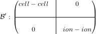(27)

This works, however, the process needs a duplication of ′. An equivalent, but more efficient approach, which may or may not have been the intended interpretation of the paper (Householder transformations are never mentioned explicitly, but implied) is to perform the extraction of the basis vectors from the cell-cell and ion-ion subspaces separately. These vectors can then be combined into one basis matrix which, while a different basis than would be obtained in the former approach, still spans the complete sampled subspace.

A caveat is that typically there are fewer cell vectors than we have updates, for this reason it makes sense to explicitly construct a temporary matrix of the cell-cell block of ′ and to perform an SVD on this 9 × 9 partition before proceeding to take the QR / SVD approach on the remaining ion-ion partition.

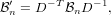
The next N² matrix to be eliminated from the routine is the mass scaling matrix, since this is a diagonal matrix :

(28)

it can be simply stored as a vector and each element multiplied by its corresponding row in Z, as the Hessian matrix in reduced coordinates called for by Pfrommer needs to take the form:

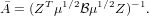(29)

NB. Pfrommer uses Y in place of Z, which was prohibited by the use of Y for gradient updates in the LBFGS formalism.

Although Z acts as a linear map from the full N × N space, to the reduced coordinate space of dimension M × M (and so A and the multiplications involved in its construction can be performed in a linear-scaling amount of memory), it is worth noting that since we have a rank-n correction to a matrix, ₀, we could use the Woodbury formula mentioned earlier.

(30)

where the mass scaled basis, Z = μ^1∕2Z.

(31)

3.0.3 Extraction of Elastic Properties and Phonon Modes

At this point, all of the O(N²) matrices should have been eliminated. This is not the case, however. The original geometry code stores A in an N² matrix to be sure that it doesn’t overflow. With a fixed history length, we shouldn’t have this problem, as we can guarantee that A ≤ m because of the rank-nullity theorem. With this simple change, the whole routine scales linearly in memory.

One further problem, unassociated with scaling but important from the perspective of implementation of the Pfrommer scheme with LBFGS is that Pfrommer puts the cell-cell segment of _n into Voigt-space. That is, symmetry of the cell system is explicitly imposed; however, symmetry of the matrix is lost. For the sake of reducing the size of _n by 3, this was not considered a good idea, since there is no mapping between the symmetric product of LBFGS and the Voigt cell.

In switching from a 6 × 6 cell to a 9 × 9 cell, there is an important issue of stride, because the latter case properly represents the rank-4 strain tensor and the elements to sum for the bulk-modulus are 1,5,9 rather than 1,2,3 for the rank-2 symmetrised strain tensor in Voigt notation.

Furthermore, it was found that in extraction of the Phonon-frequencies, a Cholesky decompostion could be employed to improve the efficiency of the procedure.

4 Measurement

In order to measure the memory requirements of the old and new code, the Linux virtual file-system in /proc was used to find the peak memory usage before and after calls to the geometry code. The file /proc/self/status was read in, and the lines beginning ’VmPeak’ and ’VmExe’, were used to find a peak memory estimate at that point in the calculation : total memory used = VmPeak - VmExe. VmExe is the size of the executable and irrelevant to this exercise (including it will introduce error to the measurement, since the binary with LBFGS is larger than that without).

Now that a way has been established to find the memory use of all the code, to find the memory used by the geometry code only is a matter of performing the procedure at the beginning and end of the parent geometry routine (geometry_optimise) and then : geometry memory = final memory - initial memory.

Measuring the time taken by the code is a similar process. However, rather than using the proc vfs, the MPI wall-time routine (MPI_Wtime) was used. The time taken in the function evaluation was subtracted as this is disjoint from the amount of time spent in the geometry module. The number of functions evaluations was recorded. For unbounded LBFGS runs, however, as this would effect the overall time taken with respect to BFGS.

An important artefact of measurement was that systems even mildly perturbed could take different routes though configuration-space and even to distinct minima. For this reason, it was important to be careful what was compared directly. Different LBFGS history lengths will inevitably lead to different paths, since the Hessians give unequal curvatures at each point in the space, which leads to differing search directions.

Comparing the memory usage is a perfectly reasonable thing to do, however, since for a fixed history length, the amount of memory required is independent of the path to convergence.

5 Implementation

Because the objective of the project was to improve memory scaling, this was kept in mind throughout the work and affected every aspect of the implementation, but to keep performance good, BLAS and LAPACK were employed wherever possible. In fact, the only significant operation which does not rely on these libraries is “geom_init_H_mul”, this is the bespoke multiplication routine for a symmetric, penta-diagonal band matrix by a general matrix. It is only called 3 times in the code, however.

The first objective of the project was in fact to replace the Fortran 90 intrinsic matrix functions (matmul) with their BLAS equivalent. As the Hessian (and its inverse) are symmetric, DSYMM and DSYMV could be employed. These initial changes made some small but not insignificant improvements to the performance:

The second objective was to implement the basic LBFGS algorithm within CASTEP. This was achieved swiftly in accordance with Byrd, et al. The original code used intrinsic matmul functions to transform from positions to forces using a multiplication by the Hessian matrix eq. (5) or backwards by multiplying the force vector by the inverse Hessian matrix, for example in the constraints section.

The second important aspect of the original code was in the construction of the Hessian matrix. The changes in position and force vectors at each iteration through the main loop would be used to form a rank-2 update matrix eq. (6), which is known as the BFGS update and is applied to the stored Hessian matrix. This was all performed within one subroutine.

In the implementation of basic LBFGS, it was determined that a routine should be developed to perform the former operation, that is to multiply the Hessian matrix by a vector without ever constructing it explicitly. This routine could be called instead of a matmul whenever this operation was required and perform as a wrapper to the BLAS, DSYMV routine whenever BFGS was invoked. Two mutually exclusive logical variables were added to the module global declarations: do_bfgs and do_lbfgs which would determine which set of operations to perform within this routine and also any others which were added or extended to offer both BFGS and LBFGS functionality. The matrix-vector multiplication routine was implemented as in algorithm (2), which performs the operation presented in eq. (6), with consideration of the 2 × 2 block diagonal (with one block zero) structure of the middle matrix, W, for maximum efficiency.

Since there was already a routine to perform the BFGS update, this was not re-written, but extended for LBFGS using the global flags to identify when a full Hessian would be present and when only update vector storage would be available (LBFGS). This just means appending the latest position and force update vectors to the respective update history matrices, of dimension n×m. For the sake of efficiency, the R matrix, eq. (14) is also stored, since this is only m × m dimensioned and can be updated efficiently with one BLAS level 3 operation: the multiplication R by the m×n position update matrix, S^T and a further BLAS level 2 operation in the multiplication of this matrix by latest gradient update vector, to give the latest, right-most column of the matrix. The final operation is to calculate the diagonal element of this column, which is a BLAS level 1 operation and hence gives the right-triangular structure of R with a new column.

In terms of computational efficiency, the BFGS update routine does O(N²) operations, whereas the LBFGS equivalent does O(M²N). Some speedup should be seen from this alone (assuming, as always, an unbounded history length), however the BFGS update was performed with scalar operations and hence the new vectorised LBFGS code should be further improved.

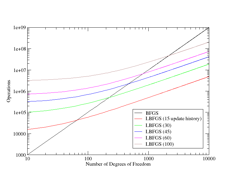
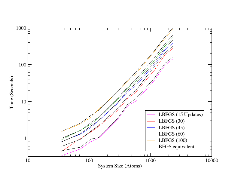
For the overall performance scaling of the scheme, there has to be some consideration for the scaling of not just the BFGS update, but for the application of the matrix to a vector (the former point above), since much of the operations have moved there from the update itself (BFGS was just a single O(N²) matrix-vector operation). From the algorithm this presents an operation count of 2NM² + 2MN + 3M³ + 2M² + 6N. Which is highly dependent of the number of stored vectors. The prefactor for BFGS was determined from the original code to be 10, by counting the number of scalar operations in the loops, so plotting 10N² versus the LBFGS count, we can compare the theoretical performance scaling, which as with the memory, is linear, but this time with a much larger pre-factor. The result of which is that in terms of performance, the scheme is beneficial for large systems, per iteration, but only for large systems with relatively short history lengths (see fig. 5). Also, this does not take into account the difference in the number of iterations to convergence which may be observed between BFGS and LBFGS with a fixed history length. This will be far more significant to the net calculation time, since performing each step requires an energy and force evaluation, which are vastly more intensive than the geometry code, with the possible exception of the Hessian analysis (SVD).

In the Hessian analysis part of the code, there was vast scope for improvement. While the main aim of the exercise was to make it linear scaling in memory, down from storing a further 6 N² matrices, because of how it was implemented, large performance gains could be possible due to the reduction in number of operations.

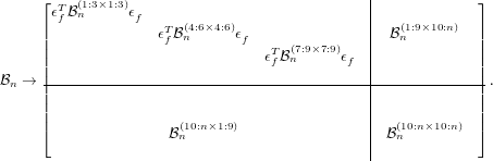
Firstly the basis of the Hessian update had to be computed, as in fig. 3, which is detailed algorithmically here:

Function f : ℝn → ℝn, Zbasis(′)
U1:n×1:2m	=
	= qr(U)		DGEQRF
C1:2m×1:2m	= RW		DTRMM
C	CR		DTRMM
	= spectral(C)		DSYEVD	(2)
v	= pivot(Λ)		algor_sort
∀i ≤ 2m : Λ(i)	Λ(v(i))
∀i ≤ 2m ∧ Λ(i) > 0 : P1:n(i)	P1:n(v(i))
Z1:n×1:l	= U1:n×1:2mP1:2m×1:l		DGEMM
End Function

Following the extraction of a basis in the update space, it must be applied to the full Hessian to form A, which is the Hessian in reduced coordinates, of which there are l ≤ 2m, by the rank-nullity theorem. There are two ways to perform this procedure. The naive way is simply to multiply out eq.(30) and invert, the more sophisticated way is to use the Woodbury formula (eq.(8)), since we want the inverse of a sequence of rank updates to a matrix. Either way, the procedure involves two parts, the change of basis in the initial inverse Hessian (₀) and in the update to it (′). 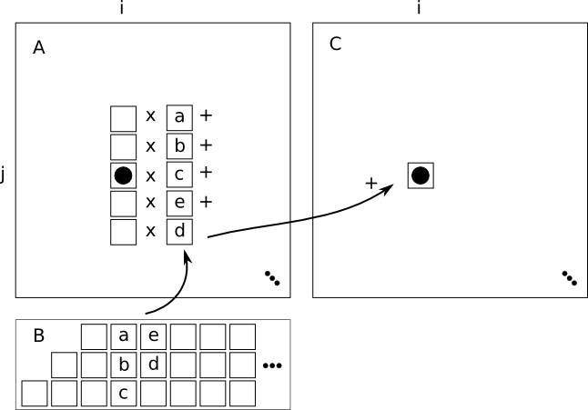For the complete expression, we may use the Woodbury formula, but for the first part of it, there is a general, dense n × l matrix multiplying a symmetric, penta-diagonal band matrix. There is no BLAS or LAPACK routine to perform such an operation, so one was written: fig. 6. NB: keep in mind the structure of the band matrix in storage is as in (19).

For the whole expression, the Woodbury formula is implemented straightforwardly with a series of general matrix multiplications (DGEMM), the above routine and the CASTEP and ONETEP wrappers to the LAPACK general inversion routines (i.e. DGETRI).

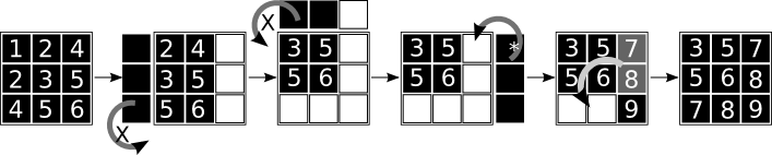
Further changes to the code involve restart code which simply makes certain that all of the correct arrays have been allocated and initialised, routines to remove and add updates to the decomposed Hessian representation using eoshifts, as described in fig.1 and fig.2.

A further essential part of the new code was a routine for resizing all of the arrays in the decomposition without losing any data. This was not for the normal use case where a fixed-history length would be employed, but for an unbounded calculation, to maintain compatibility with the old BFGS. This is simply a matter of allocating a temporary array with the old size, copying the data into it, deallocating the array, reallocating it with the new size, copying it back from the temporary array and then deallocating the temporary array. This was done for every array and works to up or down-scale arrays based on arguments.

Since the codebase in ONETEP is based on that in CASTEP, there was very little extra to do and all of the LBFGS and Hessian analysis is shared between them. The only difference is in the checkpointing and restarts, where ONETEP uses a mock CASTEP “model” in the geometry_optimisation module and this had to be updated along with some small changes to the routines due to the different routines used for inverses and sorting between the two codes, for instance.

6 Results and Comparisons

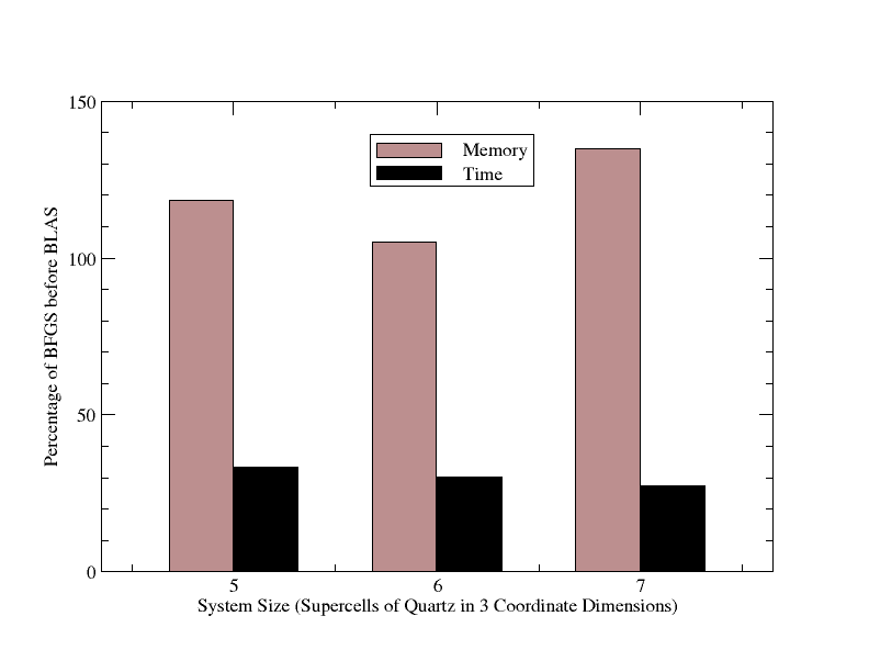
A set of test cases of various numbers of atoms were run with the original BFGS code and with the new LBFGS code under both CASTEP and ONETEP. Both castep and ONETEP use exactly the same geometry optimisation code, differing only in the energy and force solvers. Therefore the code was tested for a variety of supercells of quartz with noise in the ionic positions and cell degrees of freedom. This was then regression tested against the CASTEP and ONETEP test-suites for geometry optimisation to make certain that the same results were obtained pre and post LBFGS. The memory footprint was measured as mentioned earlier in the report. This was performed for several LBFGS history lengths and averaged over 3 runs.

The whole process was performed with and without the extraction of Physical information for reinitialisation (Bulk moduli and Phonon Frequencies), to highlight the particularly good improvement in this area.

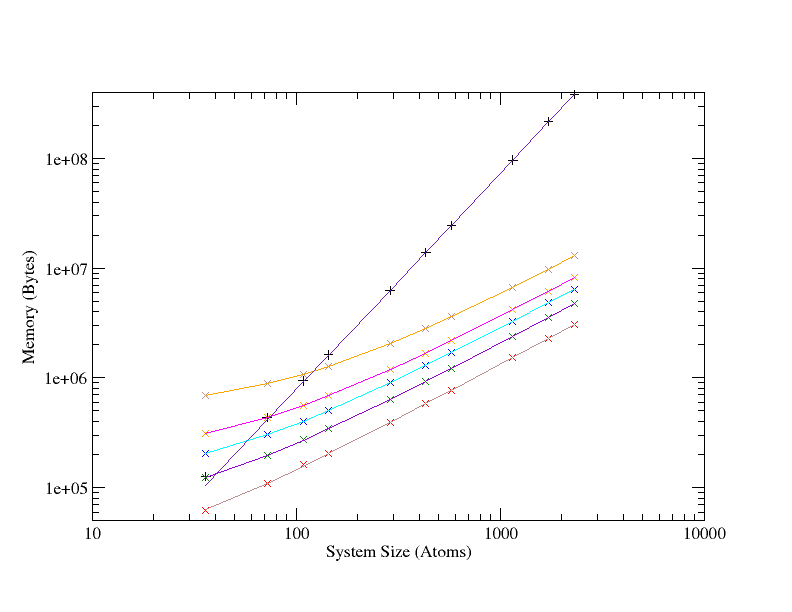
LBFGS shows linear scaling properties compared to the quadratic scaling of BFGS; figure 7. The LBFGS line for 100 updates (the uppermost line) intersects with the BFGS line at roughly 100 atoms, as would be expected.

For the largest system shown on the graph a 100 element history length LBFGS calculation requires roughly 10 MB, whilst the BFGS run consumes more than 300MB.

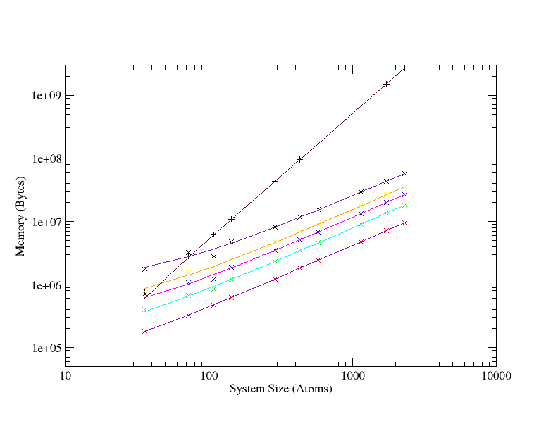
Similar characteristics are seen when the routines for extracting elastic properties and phonon modes are switched on, in that the same quadratic to linear improvement in scaling is seen between BFGS and LBFGS, however the raw difference in memory usage is much increased. For instance, taking the largest (2300 atom) system, once again, that with a history length of 100, LBFGS peaks at under 60 MB, while BFGS hits 2.5 GB.

It is worth mentioning at this point that with the original code, the N² arrays were duplicated on each MPI image, so on a system like HECToR phase 2B with 24 cores per CPU, in the pathological case, when each node is fully loaded, a geometry optimisation would require 2.5 × 24 = 60 GB. Which is well outside of the 32 GB available per node, besides which, there is also the wavefunction overhead in CASTEP which is outside the geometry module and that from the operating system, etc. As such, a geometry optimisation with a Hessian analysis in the thousands of atoms is now feasible on HECToR without seriously under-loading nodes and hence wasting AUs.

There are other considerations, of course, such as the time to science. While new calculations are now possible; systems in the tens of thousands of atoms are now entirely reasonable for geometry optimisation with CASTEP and an LBFGS calculation with a history-length of 15 will only reach 2.5 GB of memory at 600,000 atoms, such a short history length was found to converge slowly with respect to BFGS in practice (but always to converge).

History lengths of 30 or more were found to be good. 30 in particular was picked out as a good compromise.

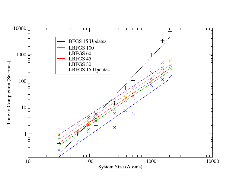
Time taken to convergence is a poor measurement for comparison, because altering the number of stored updates to the Hessian will change the search directions and hence the path to convergence, which is ultimately an unfair test. Instead, fixed history lengths were tested, followed by the Hessian analysis procedure. This means that up to the point of analysis, the calculation followed the same trajectory and at this point, the timing data for the analysis can be fairly compared.

7 Conclusions

All of the project goals were met; LBFGS was implemented in the Geometry module for both CASTEP and ONETEP, the original code was altered to use BLAS instead of Fortran 90 intrinsic functions such as matmul, the Pfrommer (re)initialisation was preserved in the LBFGS implementation and the process to extract elastic properties and phonon modes from the Hessian for use in the Pfrommer initialisation was upgraded to work with the LBFGS decomposition of the inverse Hessian and to perform the process in O(N) memory compared with the quadratically scaling memory requirements of the original code.

Further to this, the memory associated with the geometry code in CASTEP is no longer duplicated (along with all of the arrays), on every MPI image. The result is that while the current trend in HPC is more cores per node and hence less memory per core, the geometry code in CASTEP will be able to use all of the memory of a node.

It was found that for large systems, the new implementation allowed for BFGS cycles to be performed, where previously they were infeasible due to the storage requirements of the Hessian sized objects. Typically, storage was decreased by several GB for systems of the order of hundreds of atoms. Of course, the number of BFGS steps stored is crucial both to good performance and to a reasonable memory footprint. It is hoped that the memory estimate routine modifications will allow dry-run calculations to find optimum values for production runs.

All of the project goals were met; LBFGS was implemented in the Geometry module for both CASTEP and ONETEP (tasks 3,5), the original code was altered to use BLAS instead of Fortran 90 intrinsic functions such as matmul (task 2), the Pfrommer (re)initialisation was preserved in the LBFGS implementation and the process to extract elastic properties and phonon modes from the Hessian for use in the Pfrommer initialisation was upgraded to work with the LBFGS decomposition of the inverse Hessian and to perform the process in O(N) memory compared with the quadratically scaling memory requirements of the original code (an improvement on the goals of task 4).

8 Project Evaluation

The project proceeded at a fast pace initially, as the goals of adding BLAS instead of Fortran intrinsic routines and basic LBFGS functionality were completed. At the beginning of the work on the elastic properties and phonon mode extraction procedure for Pfrommer-style reinitialisation, it became clear that the task would not be trivial. The work was finally completed, through concentrated effort a little behind schedule. I hope that this work will be as beneficial to those doing geometry optimisation as it was to myself.

9 Further Work

While outside the scope of this dCSE, potential further improvements were identified as a matter of course. Firstly, in constrained cell minimisation there is scope for a better line-search. While the current method of trial steps often works, it is believed that with further work, a better solution can be found which could potentially save a large number of HECToR AUs for such calculations.

10 Acknowledgements

I would like to thank Matt Probert and Phil Hasnip of the University of York, and Craig Lucas and Christopher Armstrong of NAG (UK) for their continuous encouragement, support and ideas throughout the project, without which it would not have been possible.

This project was funded under the HECToR Distributed Computational Science and Engineering (CSE) Service operated by NAG Ltd. HECToR - A Research Councils UK High End Computing Service - is the UK’s national supercomputing service, managed by EPSRC on behalf of the participating Research Councils. Its mission is to support capability science and engineering in UK academia. The HECToR supercomputers are managed by UoE HPCx Ltd and the CSE Support Service is provided by NAG Ltd. http://www.hector.ac.uk

References