
Abstract
In this report we describe performance optimisations carried out on CARP (a cardiac simulation code) as part of an 8 month dCSE project. We have implemented a parallel mesh decomposition scheme and asynchronous parallel output that give performance improvements of around 250% for small systems, rising to 1800% for large simulations. As a result of these gains, a monodomain simulation of a human heartbeat (1 second activity) is possible in under 5 minutes: before this work began, the same simulation would take around 75 minutes to complete.
We also detail how further performance gains might be achieved in the code in response to benchmarking of the newly optimised simulations.
The Cardiac Arrhythmia Research Package (CARP) is a widely-used software package designed for large-scale simulation studies of hearts. The aims of these studies are to provide detailed personalised therapies for treatment of medical conditions. The areas where incorporation of in-silico modelling into the clinical workflow are feasible include cardiac resynchronization therapy (for treatment of arrhythmias); drug trials (looking for possible side-effects); and development of better defibrillators.
The simulation requires a model of a heart, typically obtained from the discretisation of an MRI scan (Bishop et al., 2009), as input. CARP has been developed to target a number of different architectures. Compile time options can be used to choose the level (if any) of parallelisation: a single serial processor; openMP parallelism of some loops; off-loading some computation onto GPUs; massively parallel MPI. In this project, we have only considered the MPI-parallel code. Some of the optimisations we have implemented – most notably the mesh decomposition – should also be applicable to the other compile-time targets.
Profiling work carried out prior to the start of this project identified two main areas which we needed to address to allow CARP to run efficiently on large HPC platforms. The parallel decomposition scheme results in high levels of load imbalance giving poor performance. Our first objective, therefore, was to improve the decomposition used. In addition, further profiling identified the output routines as a signficant bottleneck in simulation of large systems. We therefore also needed to optimise the output routines for use on thousands of cores.
CARP solves the cardiac bidomain equations (Plonsey, 1988) numerically on a fully unstructured 3-dimensional finite element mesh. The differential operators are discretised on the mesh and the kernel of the simulation loop thus becomes the solution of large sparse linear systems of the form
|
| (1) |
An operator-splitting approach is applied to the bidomain description resulting in three decoupled equations. The complete solution is found by leap-frogging between these decoupled components. The three equations consist of a linear elliptic PDE, a linear parabolic PDE and a set of non-linear ODEs. Solution of the elliptic PDE dominates the computational time (Linge et al., 2009).
The heart is divided up into a finite number of small sections forming the input mesh. Each section is referred to as an element and the corners of the elements are vertices. To form the shape of the heart, each vertex has a fixed position in space. Although they are somewhat larger, we can think of the elements as approximating the individual cells that constitute the heart. The aim of the simulation is to solve for the electrical potential on each of these elements. This potential causes the contraction of the heart muscle leading to a heartbeat.
The parallelisation strategy CARP employs is to divide this finite element mesh into separate regions. The bidomain equations are then solved on these regions, data are communicated between these regions which are each solved on a separate MPI process when necessary. In our linear system picture of the problem, this corresponds to storing a subset of matrix rows and columns locally on each process. Any elements in the matrix outwith this block-diagonal decomposition will require communication. For good parallel load balance, the decomposition of the input mesh into separate regions is crucial. In the next sections, we describe CARP’s existing decomposition scheme and the new scheme we have implemented.
The CARP code currently employs a vertex-based decomposition of the input
mesh. Each process considers a contiguous chunk of vertices to be local and uses
a simple tie-breaking rule to decide if an element is also local. If there
are p processes and N vertices, then process j has a local set of vertices
V j =  . Each element is defined by a set of vertices
v = {v1,v2,…,vn}. An element is considered to be local to a process j if
min v ∈ V j. This method leads to a very even distribution of the number of
vertices between processes.
. Each element is defined by a set of vertices
v = {v1,v2,…,vn}. An element is considered to be local to a process j if
min v ∈ V j. This method leads to a very even distribution of the number of
vertices between processes.
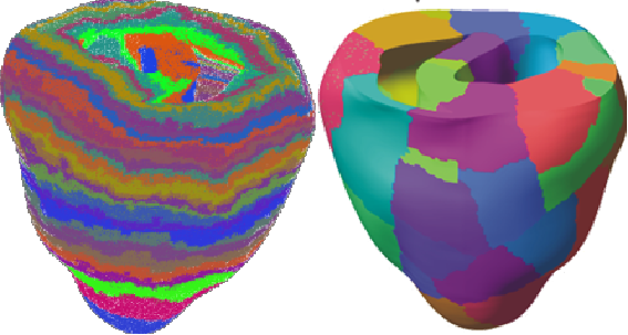
Unfortunately, the distribution of elements each process considers to be local can be very unbalanced with this scheme. Furthermore, this partitioning technique makes no attempt to minimise interface size, leading to high communication costs on parallel systems. See figure 1 for an example of the partitioning of a small heart mesh obtained with this scheme.
When we construct the linear systems defined by this mesh, local vertices define the local rows in the sparse matrix. An entry appears at Aij in this matrix if vertices i and j are in the same element. The unbalanced element ownership means that some parts of the matrix are much denser than others; the large interfacial area in the partitioning results in many off-block-diagonal entries in the matrix. Matrix-vector multiplications using the partitioning require a large amount of communication. These facts exhibit themselves as poor parallel load-balance and hence poor scaling behaviour.
Achieving good load balance requires that we partition the mesh in a more efficient manner than the existing CARP code. To do this, we employ an element-based, rather than vertex-based, decomposition technique. Our aim is to divide the mesh into a set of equal-sized domains, minimising the interfacial area. This is a graph partitioning problem. We construct the dual graph of the mesh: each element in the mesh becomes a node in the graph and each face shared between elements a link (see figure 2).
We then find a minimum cut k-way bisection of this graph.
Finding optimal k-way bisections of graphs is an NP-hard problem (Garey and Johnson, 1979), and the development of algorithms to approximate the best solution is an open and active research area. Fortunately for us, a number of high-quality software libraries exist for partitioning graphs in this manner. We have chosen to implement an interface to the parallel library ParMetis (Karypis et al., 2003; Schloegel et al., 2002). Although only a single library was used, most of our implementation is library-agnostic. To interface with different libraries such as PT-Scotch (Chevalier and Pellegrini, 2008), one must provide a function to translate CARP’s mesh description into the mesh description required by the library. The code then assumes that this library call returns a distributed vector indicating which partition each local element should belong to.
Once a good partitioning of the mesh has been obtained, we need to do two things. First, we redistribute the element data based on the new partitioning. To do this, on each process we pack a buffer containing the elements to be distributed to all other processes. These buffers are exchanged with MPI_Alltoallv. We then unpack the buffer into new element data structures.
Secondly, we must renumber the vertices according to the new distribution of elements. This is to ensure that processes have a contiguously numbered set of local vertices. Renumbering the vertices requires a little thought. As figure 2 shows, vertices on the interface between partitions could be assigned to more than one possible partition. The interface elements become more important for load balance as we increase the number of processes we run the simulation on: the surface-to-volume ratio increases and a good tie-breaking rule for ownership of the interface vertices is crucial. We have implemented two different renumbering algorithms in CARP which may be selected by the user at run time.
This scheme uses a very simple tie-breaking rule, vertices on a boundary between a set of partitions are always assigned to the lowest-numbered partition. This renumbering scheme is carried out in serial by looping successively over each process and renumbering as yet unseen vertices sequentially. This method has two drawbacks: it typically assigns more vertices to low-numbered ranks than high-numbered ones (due to the choice of tie-breaking rule); additionally, the algorithm does not scale at all.
To overcome these problems, we have also implemented a parallel renumbering scheme that does a better job of balancing the boundary vertices between partitions. This algorithm is slightly more involved than the serial one, the basic idea is to work out which vertices live on only a single partition and which are interfacial. We then use a simple heuristic to assign interface vertices to an appropriate partition.
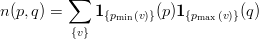
Let pmin(v) and pmax(v) be the minimum and maximum numbered partitions a vertex v appears on. For example, if vertex v appears in elements on partitions 2, 4 and 7 then pmin(v) = 2 and pmax(v) = 7. This allows us to find shared (interface) vertices. This heuristic is not perfect: we have assumed that only two-partition interfaces are important.
On each partition p we now calculate n(p,q) the number of vertices shared between partitions p and q (p ≤ q):
 | (2) |
where
 | (3) |
is the indicator function.
Of these shared vertices, partition p owns the first
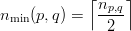 | (4) |
and partition q owns the subsequent
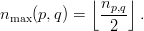 | (5) |
Each partition p is now able to calculate the number of vertices it owns
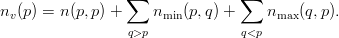 | (6) |
We now communicate the number of owned vertices between all partitions to calculate the starting index of the new numbering on each partition. On each partition, we then loop over all vertices and renumber those vertices we own (according to the above rules) linearly. Finally we communicate the partially filled in remapping vector between all partitions and renumber the vertices in the element datastructure.
This algorithm requires two calls to MPI_Allreduce, one to MPI_Exscan, one to MPI_Allgather and one to MPI_Allgatherv. This is in contrast to the serial (simple) renumbering which requires as many MPI_Send calls as there are partitions and then one MPI_Bcast. In practice, for a system with 150 million elements, we find the parallel renumbering takes around 20 seconds (irrespective of number of processes). The serial renumbering takes around 50 seconds on 256 processes rising to almost 600 seconds on 8192 processes. As a result, we have made the parallel renumbering scheme the default option.
Once the mesh has been read in and partitioned, CARP constructs a sparse matrix representation of each of the differential equations to be solved. The bulk of the work in solving these equations is handed off to the parallel library PETSc (Balay et al., 1997, 2008, 2009). In particular, the elliptic and parabolic PDEs are solved using preconditioned conjugate gradient. The ODEs are solved using an explicit method. The parabolic PDE may also optionally be solved using an explicit method. We elaborate further on this below. See Bordas et al. (2009) for a recent review of the techniques used for solution of these equations.
Consider a linear system
 | (7) |
with  a vector of N unknowns. If A is symmetric positive definite, the conjugate
gradient method is guaranteed to converge to the correct solution to this equation
in N steps. On a computer, due to the inadequacies of floating point
representation, we will never converge to exactly the right solution. Instead, we
stop iterating the method when the difference between our proposed solution and
the “correct” answer is less than some tolerance t. That is, we iterate
until
a vector of N unknowns. If A is symmetric positive definite, the conjugate
gradient method is guaranteed to converge to the correct solution to this equation
in N steps. On a computer, due to the inadequacies of floating point
representation, we will never converge to exactly the right solution. Instead, we
stop iterating the method when the difference between our proposed solution and
the “correct” answer is less than some tolerance t. That is, we iterate
until
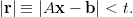 | (8) |
The number of iterations the algorithm takes to converge is an increasing function of the condition number of the matrix A (the ratio of the largest to the smallest eigenvalue). To converge in a small number of iterations, we therefore want our matrix A to have a small condition number.
Consider the equation
 | (9) |
where M is a non-singular matrix. This is mathematically equivalent to equation 7, but may well have different convergence properties on a computer. For example if M = A-1 then MA = I is the identity matrix and the conjugate gradient method will converge in a single step. The application of a matrix M to a linear system of equations to speed convergence is known as preconditioning.
Ideally, we would precondition the system using M = A-1, since in this case the solution is immediately obtained. Unfortunately, constructing the inverse of a matrix is a computationally expensive problem. Furthermore, the inverse of a sparse matrix is in general dense: if our linear system is large, we may not have the memory necessary to store the inverse. Instead, we aim to find a matrix M which is cheap to compute and a reasonable approximation to the inverse of A while remaining sparse. We precondition our linear system with this matrix M to decrease the condition number of the system, decreasing the number of iterations to convergence.
Obtaining good performance for the implicit solvers is therefore a two-step process. Firstly, decomposing the problem in the correct way to ensure good load balance. We have described our approach here already. The next step is to choose a good preconditioner. We cover this in the following section.
Multigrid preconditioners have been shown to give good convergence behaviour
for elliptic PDEs (Stüben, 1999). The idea is to take the fine-grained problem and
coarsen in some specific way to produce a smaller problem. That is, from the
linear system A =
=  we produce the coarser system Ac
 =
=  which is
computationally cheaper to solve. This system is iterated and the solution is
then interpolated back onto the original system. Using multigrid as a
preconditioner for solving a linear system works in a similar manner. We
obtain a coarse approximation to the inverse of A and then interpolate this
result onto the original problem size to obtain our preconditioning matrix
M.
which is
computationally cheaper to solve. This system is iterated and the solution is
then interpolated back onto the original system. Using multigrid as a
preconditioner for solving a linear system works in a similar manner. We
obtain a coarse approximation to the inverse of A and then interpolate this
result onto the original problem size to obtain our preconditioning matrix
M.
For best performance, some kind of geometric multigrid scheme should be employed. However, these require both significant expertise in numerical analysis and parallel programming and must furthermore be tailored to each individual problem (Ainsworth, 2010). Algebraic multigrid (AMG) methods are an alternative approach which use information in the sparse matrix to construct the various different coarsened levels, see Stüben (1999) and Falgout (2006) for detailed introductions to the technique. These are a more generic solution which trade off performance for generality. A number of high performance parallel multigrid implementations exist, we have focused predominantly on that provided by hypre (Falgout and Yang, 2002).
One issue, in particular, that multigrid implementations have on parallel systems is that the coarsening process tends to lead to a relatively dense matrix. If not in terms of the total number of non-zeros, then certainly in terms of the process sparsity pattern. As a result, unless parameters are picked carefully, the coarse matrix multiplication can require alltoall-like message passing: even if the original matrix is very sparse. Choosing a set of parameters that give good performance is somewhat problem-specific.
CARP’s parameter set for the hypre AMG preconditioner was previously selected on a 16 processor system. We have reinvestigated the choices and have obtained a set of parameters that exhibit better performance on large systems. The PETSc solvers we use have the option to select at run time between a large number of different preconditioners. In addition to selecting a good set of parameters for the hypre AMG preconditioner, we have also studied the performance of an alternative multigrid implementation provided by the Trilinos package. In addition we have looked at the performance of simpler block Jacobi preconditioning. We do not report full results for these implementations. For our problems, we find that the Trilinos multigrid preconditioner has the same scaling behaviour but is a factor of 3 slower than the hypre AMG. The block Jacobi preconditioner is more scalable than AMG, but does not speed up convergence enough. At low core counts, AMG is much faster (around a factor of 20) than block Jacobi; for large numbers of cores, the difference is much smaller (only a factor of 1.5 or so).
We come to the detailed performance results later, the take home message is that, for the moment, hypre’s AMG implementation produces results the fastest. The set of AMG options we have settled on is:
Although it is recommended to choose a strong threshold somewhat above 0, we have found that for our system, a strong threshold of 0 gives best absolute performance and does not negatively affect the scaling behaviour of the code.
As we have mentioned previously, the generic problem with AMG preconditioners is that the coarsening operators can easily produce a comparatively dense matrix at the coarse level. This then requires a much larger amount of communication than a sparser matrix, which hinders the scalability of matrix-vector multiplies. The options we have chosen attempt to maintain the sparsity of the coarse-level matrices.
For the parabolic problem, we use a block Jacobi preconditioner and use incomplete cholesky factorisation to find the approximate inverses of these blocks. The idea here is to remove the need for communication during the computation of the preconditioning matrix. Recall that our parallelisation strategy ensures that process i has ni contiguous local rows of the matrix A. The diagonal block of size ni × ni is therefore local to a process i. We throw away non-zeros of A outside this block diagonal structure to form a new matrix
 | (10) |
Where Ai is a sparse matrix of order ni. The inverse of each Ai may be computed independently to form Ã-1. Since the inverse of a sparse matrix is in general dense, we do not even compute the full inverse of Ai explicitly. Instead we use incomplete factorisation, typically this is implemented by dropping non-zeros such that the sparsity pattern of Ai-1 is the same as that of Ai. Application of Ã-1 to our linear system should require no communication, since off-diagonal (non-local) elements will be multiplied by zeros.
Multigrid methods can also be used to accelerate the convergence of conjugate gradient when applied to parabolic PDEs. Our problem here is no exception. We have made some numerical studies of the performance of the same multigrid preconditioner used for the elliptic PDE. Although the number of iterations to convergence is much lower, the cost of each individual iteration is very much higher. The accelerated convergence rate is not enough to overcome this higher cost. As a result multigrid preconditioners give a longer time to solution than the block Jacobi preconditioner we have settled on.
The ODEs to be solved for CARP are entirely local. They are used to evolve ion levels at each grid point: this affects the conductivity of the material for subsequent timesteps. As a result, good load balance just requires that each process have an equal number of ODEs to solve. In addition, to remove the need for communication of the results, we require the set of ODE points to be the same as the local set for the PDEs. The natural solution to these constraints is just to use the same partitioning of vertices for the ODEs as for the PDEs. This way we have both good load balance and good data locality.
Since the ODEs are entirely local and require no communication, they should scale extremely well. In practice, we found that the scaling performance was much worse than expected. The reason for this is an example of why it is imperative to profile to find hotspots, rather than assuming one knows which parts of a code will be fast.
The data from the ODEs is stored as a distributed vector: the ionic levels at each vertex. The original code used PETSc routines for setting values in distributed vectors. On each process, we set values in the distributed vector, and then call routines to reassemble the data.
PETSc allows any process to set any element of a vector, the assembly calls ensure that the vector ends up in the correct state. To deal with this generality, the assembly step of the code requires global communication even if all values have only been set locally. As a minimum, one call to MPI_Allreduce is required to ensure that all processes agree on how they are adding values to the vector (insertion of new elements or addition to existing elements). This has scalability implications at large process counts. Since we know that these operations are purely local, we can replace the general PETSc machinery with a more scalable solution. PETSc allows us to get at the local backing store of a distributed vector, so we can set local elements by modifying this data. Setting local values is simply:
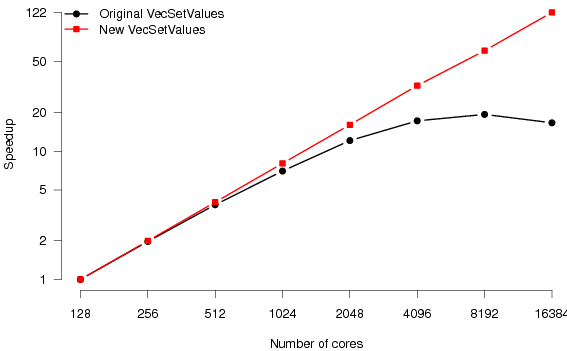
This method has none of the scalability problems of the generic version, and hence as long as we have good load balance, the ODE solve is now almost perfectly scalable. Figure 3 shows the effect of this change on the scaling behaviour of the ODE solve.
As we saw in section 4.4, unexpected portions of the code can exhibit performance problems at scale. In this section we describe the approach we have taken in fixing another of these issues, namely the output system.
Other than fixing any performance issues, our primary concern in this set of code modifications is ensuring that end users do not have to change any of their analysis routine. Changes that make the code run faster are good, but we have to remain backwards-compatible with existing analysis tools. Essentially, this means making the output go faster without changing the file format.
CARP’s output routines were originally written for serial output and have had parallel output bolted on to them after the fact. Most of the output consists of writing vectors describing the electrical potential defined on the grid points to output files. These vectors are written using a gather-to-rank-zero approach. That is, when output is required, rank zero writes its local portion of the data and then sequentially receives and writes data from all other processes. All processes then wait at the end of the output routine.
With this method, the time to write a distributed vector is an increasing function of the number of processes. The time to write the data to disk is a constant, but as the number of processes increases the time spent gathering the data also increases.
To remove this serial bottleneck in the code, we needed to implement parallel output routines. The distributed vector that we need to output maps quite nicely onto parallel output using MPI-IO, however, there are a number of problems with this simple-minded approach that we detail below.
Recall that one of our primary aims is to preserve backward compatibility with the existing output format. Our previous changes to fix the load balance by repartitioning the input mesh have violated this design decision. Visualisation of the data requires both the output vectors and the mesh they were generated on: the ordering of the vector indicates which point the data are defined on. The ordering of grid points in the repartitioned mesh is not the same as that on the input mesh. We have two options to solve this problem. Either, we output the repartitioned mesh for every simulation run – users then visualise the output data on this repartioned mesh; or, we map the output data back onto the input mesh before writing it to disk.
Since the repartitioned mesh can in theory be different for every simulation we run, but will hold no new information – it’s just a permutation of the input – we rejected the first solution detailed above. This leaves us with mapping the output data back onto the input mesh. This is easily done, using PETSc’s VecScatter and index set routines, but has a high communication overhead. In general, this mapping will require all-to-all communication. This is a communication-dominated bottleneck that affects the scaling performance. We therefore rejected the idea of implementing parallel output of the distributed vector using MPI-IO. Although the output itself would be parallel, we would still run into communication overhead. Instead of this we have implemented an asynchronous output scheme that blocks the computation significantly less. This output scheme can be selected by the user at run time. A command-line option can be used to specify the number of cores to dedicate to output. If zero cores are dedicated, the original output system is used.
Instead of attempting to parallelise output across all the processes carrying out computation, we have instead rewritten the output system so that processes carrying out computation do not ever write to disk. We dedicate a small number of processes to output – the exact number may be specified by the user at runtime. When an output routine is called, the distributed vector defined on the compute processes is scattered onto the output processes. At this point, the compute processes are done and can continue the simulation.
On the output processes we now map the data back onto its canonical ordering before writing it to disk. We have implemented both serial output (using the existing framework in CARP) and parallel output using MPI-IO. Figure 4 shows this process schematically.
We note that our output scheme is not truly asynchronous. In particular, although the output nodes aim to pre-post all receives for data, incoming messages will not be processed in parallel even if the matching receive already exists. The receive loop in the code looks like this:
The MPI_Waitany call effectively serialises the receipt of messages, even if the message buffer is preallocated. If do_stuff_with_data takes a long time to complete, the processes sending data will wait some time for ACKs indicating that they can release the buffer and continue (Edwards and Roy, 2010). We note that irrespective of this small issue, the improvement in IO performance is approximately a factor of 20 on large system. Where previously IO throughput was around 25MB/s, we now obtain an effective throughput of around 460MB/s for a simulation on 8192 cores.
Should this serialisation become a problem, there are a few ways we could address the issue. All of these increase code complexity, and we have found that with a suitable choice for the number of IO processes the performance is entirely adequate. For completeness, we detail other potential solutions that could be implemented should the need arise. Since we are pre-posting all the receives, the natural thing to do on the send side is to use a ready send rather than a standard send. Since in this case the receive is guaranteed to exist, the MPI implementation can potentially optimise the call. There is, however, a problem with this idea. Since the output is initiated on the compute nodes, we cannot guarantee that receives will be pre-posted unless sending an additional message from.
A option for removing the need for a message ACK is to use non-blocking sends. Our compute nodes keep track of the status of this message and MPI_Wait on it at the beginning of the output routine. This method, too, has drawbacks. We have to copy the data into a temporary buffer so that it is not overwritten by the continued computation steps.
It is worth mentioning that all the improvements detailed previously have had approximately the same cumulative effect as a one-line code change we have previously not mentioned. Again, this is an example of needing to profile code religiously to find hotspots: often in the most unlikely places.
When carrying out some initial profiling runs, we found a routine that just printed some progress statistics was taking an inordinately large portion of the runtime for large jobs. The problem was a bad interaction between the way progress statistics were printed and the filesystem implementation. Each process would enter the progress function and call
The fflush call being used so that on a workstation the user will always see up-to-date progress statistics. On HECToR, this had a terrible interaction with the Lustre filesystem. Output was effectively serialised and all other processes would block at the call. Since on a large parallel machine there is no need to view the progress statistics in real time, we removed the fflush call. Furthermore, since the statistics were identical on all processes, we now just have a single process printing statistics. Table 1 shows the fraction of time spent in output routines before and after this change for the OxfordHeart system described in section 6.2.
| Cores | Before | After |
| 32 | 0 .018 | 0 .016 |
| 64 | 0.081 | 0.03 |
| 128 | 0 .15 | 0 .081 |
| 256 | 0.16 | 0.057 |
| 512 | 0.18 | 0.058 |
| 1024 | 0.23 | 0.049 |
| 2048 | 0.5 | 0.052 |
We present results from three different systems. The first, TBunnyC1 , is a 3-D mesh of a rabbit heart with 862 515 vertices and 5 082 272 elements. The second system, OxfordHeart2 , is a more detailed 3-D mesh of a rabbit heart with 6 901 583 vertices and 40 992 163 elements (Bishop et al., 2009). The final system, HumanHeart3 , is a 3-D mesh of a human heart with 26 190 199 vertices and 152 891 134 elements.
For the TBunnyC and OxfordHeart models, we solve the full set of bidomain equations: elliptic and parabolic PDEs as well as the ODEs. For the HumanHeart model, we only solve the monodomain equations: just the parabolic PDE and ODEs. The elliptic problem is by far the most computationally expensive and would take too much time to benchmark and run for the HumanHeart system.
Figure 5 shows the scaling behaviour of the original and new CARP code. Where previously the code would scale to 64 processes, it now reaches 256. Relative to the original code, we have achieved a speedup of 2.5 in the minimum execution time for a simulation (on 256 as opposed to 64 processes).
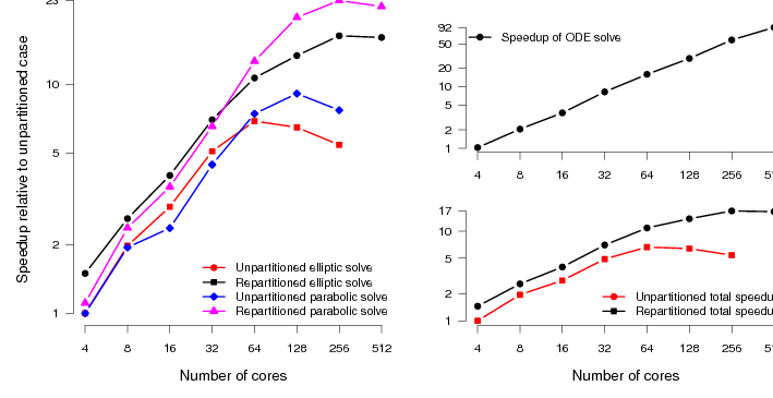
Notice that the scaling regime of the elliptic and parabolic PDE solvers is extended by a factor of around four (from 64 to 256 processors). ODE is scaling, as expected, is good for all codes. Good scaling behaviour of the ODE solver relies purely on there being an equal number of ODEs to solve on each processor since there is no communication required. Both the original CARP partitioning and our new partitioning scheme satisfy this requirement.
We expect to see slightly more scaling for the original code here, just because the system is larger than the TBunnyC mesh. This is indeed the case. However, we see roughly the same pattern (figure 6). The scaling of the elliptic and parabolic solvers, which are not well load-balanced in the original code, is poor (compared to the ODE scaling).
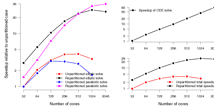
With good mesh partitioning and the addition of asynchronous output routines, the code scales to around four times as many processes with reasonable efficiency. There is also an absolute speedup over the original code of around a factor of three when run on the same number of processes. The speedup of the total simulation relative to the original code is around 740%.
Finally we look at the performance of the HumanHeart system. To the best of our knowledge, this particular model has around twice as many unknowns as the current largest studied model (Niederer, 2010). CARP allows solution of the parabolic PDE through two different methods. The first is an implicit Krylov solve using conjugate gradient. The second is an explicit solve, just requiring matrix-vector products. The explicit solution method requires both less computation and communication per timestep. The Krylov solve needs collectives to calculate dot products. However, to preserve the stability of the solution, we must reduce the integration timestep. Typically by a factor of five. So each step is less expensive, however, we need to carry out about five times as many steps. Despite these extra steps, we have found that the explicit parabolic solve is faster than the implicit solve, and moreover scales to larger core counts. Figure 7 shows the performance of the original code along with the new code on the HumanHeart. Where previously the scaling topped out at around 1024 cores, the code now scales with good parallel efficiency to 16384 cores.
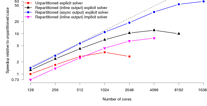
Mapping these speedups onto real-world timings, the original code would, at best, take 72 minutes to simulate 1 second of activity. The new code now takes around 4 minutes, a speedup of 1800%. This naturally opens up new avenues of research. Computational studies that would previously take weeks of compute time can now be carried out in days.
The phase 2b configuration of HECToR, a Cray XT6, has 24 cores per node arranged in two 12-core sockets, each with two 6-core chips. As of writing, the network configuration is the same as on the phase 2a machine. Each node is connected via a Cray Seastar2+ chip in a 3-dimensional torus. For a pure MPI code, this effectively means a 6-fold increase in the number of messages through each network chip over an equivalent job on the XT4. If the communications were predominantly collective, we might hope that the vendor MPI implementation would coalesce messages on an SMP node, in which case we would see a performance gain: fewer messages of a larger size typically win. For our application, most of the communications are point-to-point, so the MPI implementation cannot do any message coalescence.
The upshot of this network bottleneck is that we see much poorer performance on the XT6 than the XT4. The HumanHeart benchmark which shows good scaling behaviour to 16k cores on the XT4 does not scale much past 1500 cores on the XT6. We note that this is entirely due to the network performance. Underpopulating nodes so that the only 4 cores per node are used on the XT6 (giving the same number of cores-per-network chip as the XT4) results in entirely identical performance and scaling behaviour. As a result, we are hopeful that the upgrade in late 2010 to a Cray XE6 (upgrading the Seastar2+ network chips to Gemini) will restore performance and scaling behaviour to that seen on the XT4.
The performance improvements we have made to the CARP code have allowed for much better scalability, allowing simulation of systems that were previously too time-consuming to study. These improvements have revealed areas in the code that will require further work to fully exploit the performance increases.
The current CARP code has distributed data structures for elements in the finite element mesh, but the data defined on vertices is stored in replicated data. That is, each process has a complete copy of the vertex data. Although for the systems currently under study this lack of parallelisation has not been an issue, it is clearly not a scalable solution when moving to larger, more detailed meshes. For a cellular resolution mesh, with around 260 million elements and 40 million vertices, the replicated vertex data is minimally 900MB, this increases when partitioning is performed: we have to store further data structures mapping between intra- and extra-cellular vertex lists. In the phase 2b configuration of HECToR, we have already hit a memory wall with this scheme, since only 1.3GB are available per core.
The correct way to address this is to make the vertex datastructures distributed in a similar way to the elements. This requires a bit of thought to avoid excessive communication. We need to store the set of vertices that are local to a processes elements. This will necessitate storage of some ghost points for interface vertices, but should make the data size for vertices scalable with the number of cores.
In addition to simulating electrical activation in the bulk of the heart, for more realistic models it is also necessary to take into account the effects of the Purkinje network (Deo et al., 2008). This is a one-dimensional network of highly-conducting fibers that are electrically isolated from the bulk of the heart tissue, they are only connected at some termination points. Electrical activations travel along these fibers much faster than in the bulk, and lead to secondary activations in the ventricles.
The Purkinje system is smaller, and has many fewer degrees of freedom than the complete heart mesh. As a result, distributing the data across all computational processes would not result in good scalability.
With larger simulations possible, the amount of data that can be acquired also increases. As a result, analysis of the datasets on desktop computers becomes more and more difficult. Parallel data analysis tools are likely required. This will likely require a move away from CARP’s existing home-grown data formats to leverage existing visualisation tools such as Paraview. The VTK file formats do not allow for easy specification of 4-dimensional (space + time) datasets: the spatial structure has to be re-specified for every timestep, which is bad if it does not change. However, we note that Paraview understands the XDMF4 data format which allows attaching multiple scalar or vector properties to a fixed structure. This would allow for 4-dimensional datasets similar to the ones CARP currently uses.
With hetereogeneous (GPU + CPU) compute blades becoming a reality – Cray’s roadmap for high end systems includes GPU accelerators – offloading some of the computationally expensive aspects to a GPU is a possibility. CARP is already capable of solving the ionic models (ODEs) on GPUs when compiled for serial execution. To assess the feasibility of such an approach in a distributed memory environment, we need to consider the ratio of computation to communication. It makes no sense to speed up the solver if all the time is spent communicating data. to that end, we have performed some measurements of the ratios of compute to communication time in the time-intensive Krylov solve part of the code. Our results indicate that the compute part is well-balanced, and scales well. The communication does not perform as well. In particular, we need fast collectives for testing the convergence of the Krylov iterations. In table 2 we show the ratio of computation to communication in the elliptic and parabolic solve steps of a simulation with the OxfordHeart dataset. For the elliptic solve, we find that most of the communication time is waiting for point-to-point messages to complete in the sparse matrix-vector multiplies. For the parabolic solve, most of the communication time is waiting for allreduce calls to complete (checking for convergence of the Krylov solve). This suggests that we may be able to extract more performance from the parabolic solve if we have faster MPI collectives. Squeezing more performance from the elliptic solve at high core counts is likely to be much harder. Accelerating the computation at lower core counts using GPUs may well be a more profitable direction to take.
| Cores | Elliptic | Parabolic
|
| 128 | 3.42 | 4.94 |
| 256 | 1 .48 | 3 .18 |
| 512 | 0.53 | 1.56 |
| 1024 | 0.22 | 0.92 |
| 2048 | 0.07 | 0.35 |
The original aims of this project were to improve the strong scaling behaviour of the CARP code through better parallel decomposition and implementation of better parallel output schemes. Both of these aims have been fulfilled. The performance gains for large systems have matched the aims set out in the original project proposal. Simulation of a human heartbeat is now possible in under 5 minutes.
The results of this work have now been merged back into the central CARP repository and are now available to users worldwide. Dissemination of the work and results is ongoing, a paper was presented at CUG 2010 and a submission to PNAS is in preparation. A further paper on the work will be presented at VPH 20105 .
This work has been funded by a distributed CSE grant from EPSRC administered by NAG Ltd. Gernot Plank provided much useful direction and advice. The datasets for benchmarking were kindly provided by Martin Bishop and Gernot Plank (University of Oxford) and Steven Niederer and Nicholas Smith (University of Oxford).
M. Ainsworth. Personal communication, 2010.
S. Balay, W. D. Gropp, L. C. McInnes, and B. F. Smith. Efficient management of parallelism in object oriented numerical software libraries. In E. Arge, A. M. Bruaset, and H. P. Langtangen, editors, Modern Software Tools in Scientific Computing, pages 163–202. Birkhäuser Press, 1997.
S. Balay, K. Buschelman, V. Eijkhout, W. D. Gropp, D. Kaushik, M. G. Knepley, L. C. McInnes, B. F. Smith, and H. Zhang. PETSc users manual. Technical Report ANL-95/11 - Revision 3.0.0, Argonne National Laboratory, 2008.
S. Balay, K. Buschelman, W. D. Gropp, D. Kaushik, M. G. Knepley, L. C. McInnes, B. F. Smith, and H. Zhang. PETSc Web page, 2009. http://www.mcs.anl.gov/petsc.
M. J. Bishop, G. Plank, R. A. Burton, J. E. Schneider, D. J. Gavaghan, V. Grau, and P. Kohl. Development of an anatomically detailed mri-derived rabbit ventricular model and assessment of its impact on simulations of electrophysiological function. Am J Physiol Heart Circ Physiol., 298(2):H699–718, 2009.
R. Bordas, B. Carpentieri, G. Fotia, F. Maggio, R. Nobes, J. Pitt-Francis, and J. Southern. Simulation of cardiac electrophysiology on next-generation high-performance computers. Philosophical Transactions of the Royal Society A, 367:1951–1969, 2009. doi: 10.1098/rsta.2008.0298.
C. Chevalier and F. Pellegrini. PT-Scotch: a tool for efficient parallel graph ordering. Parallel Computing, 34:318–331, 2008. doi: 10.1016/j. parco.2007.12.001.
M. Deo, P. Boyle, G. Plank, and E. Vigmond. Role of Purkinje system in cardiac arrhythmias. In Engineering in Medicine and Biology Society, 2008. EMBS 2008. 30th Annual International Conference of the IEEE, pages 149–152, 20-25 2008. doi: 10.1109/IEMBS.2008.4649112.
T. Edwards and K. Roy. Using I/O servers to improve application performance on Cray XTTM technology. In Cray Users Group Meeting (CUG) 2010, Edinburgh, Scotland, 2010.
R. D. Falgout. An introduction to algebraic multigrid. Computing in Science and Engineering, 8:24–33, 2006.
R. D. Falgout and U. M. Yang. hypre: a library of high performance preconditioners. In P. M. A. Sloot, C. J. K. Tan., J. J. Dongarra, and A. G. Hoekstra, editors, Computational Science – ICCS 2002, volume 2331 of Lecture notes in computer science. Springer, 2002.
M. R. Garey and D. S. Johnson. Computers and Intractability: A Guide to the Theory of NP-Completeness. W. H. Freeman, 1979.
G. Karypis, K. Schloegel, and V. Kumar. ParMETIS: parallel graph partitioning and sparse matrix reordering library. University of Minnesota, version 3.1 edition, 2003. URL http://glaros.dtc.umn.edu/gkhome/metis/parmetis/overview.
S. Linge, J. Sundnes, M. Hanslien, G. T. Lines, and A. Tveito. Numerical solution of the bidomain equations. Philosophical Transactions of the Royal Society A, 367:1931–1950, 2009. doi: 10.1098/rsta.2008.0306.
S. Niederer. Personal communication, 2010.
R. Plonsey. Bioelectric sources arising in excitable fibers (Alza lecture). Annals of Biomedical Engineering, 16:519–546, 1988.
K. Schloegel, G. Karypis, and V. Kumar. Parallel statis and dynamic multi-constraint graph partitioning. Concurrency and computation: practice and experience, 14:219–240, 2002. doi: 10.1002/cpe.605.
K. Stüben. Algebraic multigrid (AMG): an introduction with applications. Technical Report 70, GMD – Forschungszentrum Informationstechnik GmbH, 1999.