Cloud and Aerosol Research on
Massively-parallel Architectures (CARMA)
Jon Gibson
Numerical Algorithms Group Ltd,
Wilkinson House, Jordan Hill Road,
Oxford OX2 8DR, U.K.
e-mail: support@nag.co.uk
28th February, 2013
Abstract
This report
presents the work carried out on the project “Cloud and Aerosol Research on
Massively-parallel Architectures”, or CARMA for short. This was a one year
distributed Computational Science and Engineering (dCSE)
support project, part of the CSE support for HECToR
[1], the UK’s national academic supercomputing service. The report first
describes the work carried out implementing a parallel iterative solver within
the Met Office Large Eddy Model (LEM). The primary purpose of this new
approach, as an alternative to the FFT-based solver, is that of enabling new
science by losing the requirement for lateral periodic boundary conditions. It
then describes the parallelisation of the code ACPIM
(Aerosol-Cloud-Precipitation Interaction Model), a process-scale model for
studying the growth and evolution of cloud from aerosols. The PI’s of the
project were Alan Gadian of the University of Leeds
and Paul Connolly of the University of Manchester.
Table of Contents
1.
Application Overview: The LEM Code
1.4.
Parallel Decomposition of the Domain.
2.
Application Overview: ACPIM
4.
The Parallel Iterative Solver
Application Overview: The LEM Code
The Large
Eddy Model (LEM) code has been developed by the Met Office as a high resolution
numerical model used to simulate cloud-scale and micro-scale atmospheric
processes, such as aerosol-cloud interactions. It implements modified Navier-Stokes equations with parameterisations for
turbulence, microphysical processes and radiation. The software is also widely
used by the scientific community outside the Met Office and is documented in [2], [3] and [4].
1.1. Basic Equation Set
As explained
more fully in [3], the LEM solves the following basic equation set, shown
using tensor notation. These equations are integrated over time using a
centred-difference scheme.
|
|
|
(1) |
|
|
|
(2) |
|
|
|
(3) |
|
|
|
(4) |
where
|
|
denotes a reference
state of |
|
|
denotes a perturbation
from the reference state of |
|
u |
is the vector flow
velocity |
|
|
is the potential
temperature |
|
|
represents all other
scalar variables |
|
|
is the pressure |
|
|
is the density |
|
|
is the buoyancy |
|
|
is the subgrid stress |
|
|
is the subgrid scalar flux of |
|
|
is the subgrid scalar flux of |
|
|
is the Earth’s angular
velocity (f-plane approximation) |
|
|
is the alternating
pseudo-tensor |
|
|
is the source term of |
|
|
is the source term of |
|
|
is the source term of qn due to microphysics |
and
|
|
|
(5) |
Calculation
of the pressure term in equation (1) requires the solution of a Poisson-like
elliptic equation:
|
|
|
(6) |
where
|
|
|
(7) |
This can be
solved by performing a Fourier transform in the horizontal to eliminate the ![]() and
and ![]() operators, solving the resulting equations
using a tridiagonal solver and then applying a reverse Fourier transform to recover
operators, solving the resulting equations
using a tridiagonal solver and then applying a reverse Fourier transform to recover ![]() . This method was the only one
implemented in the code prior to this project.
. This method was the only one
implemented in the code prior to this project.
The software
is documented fully in [4] but it is worth mentioning a few aspects of the code
here to put it in a proper context. The code is mainly written in Fortran 77
but with a few Fortran 90 features. All memory is statically allocated. The
message passing is written using a library called GCOM [5][6], a wrapper around a wrapper (called
MPL) around a small subset of the MPI library. The original idea was that the
same GCOM calls could equally interface to MPI [7], PVM [8] or SHMEM [9] libraries at a lower level, allowing
the user to easily switch between them. However, given that MPI tends to be
used universally now, the fact that GCOM only allows the programmer to access a
small subset of the overall functionality of MPI, makes it more of an obstacle
to efficient programming than anything else (not only is the entire MPI 2
functionality absent but much of MPI 1).
The approach
to version control is equally archaic. It uses a system called the nupdate source code manager [10]. The source code under this system
consists of decks (.dk files) and comdecks (.cdk files), which are
processed by running the nupdate
command to produce the Fortran source code. The comdecks, consisting of variable and common block
declarations that are common to a number of decks, get inlined
in the source code during the processing. Any modifications to the source code
need to be made by writing an update file, which is processed along with the
other files.
Jobs can be
submitted by the user using the lemsub script, which via the use of nupdate,
a default info file, a machine info file, a machine-specific run script and a makefile, updates, transfers files to the run directory,
compiles and submits a job to the batch system. This initial job is referred to
as a set-up job. A job can be set up
so as to submit a follow-on job, referred to as a chain job, upon completion and to continue to do so until a certain
point is reached in the simulation.
Parallel Decomposition of the Domain
The problem
domain is made up of IIP´JJP´KKP grid-points. The LEM integrates
the field in a succession of 2D slices in the y-z plane, moving along the
x-direction. Integration of the model equations only requires information from
up to two grid-points away so the domain can be decomposed into sub-domains
with overlapping halo regions. Figure 1, taken from [4], illustrates how the domain is decomposed in the
x-direction so that each PE holds IIP/NPES slices, along with a two-slice halo
region for each neighbouring sub-domain.
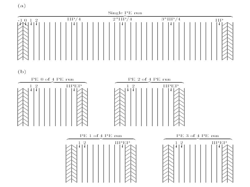
Figure 1: The LEM’s domain decomposition. Part (a) shows a single processor run. The halo slices implement the periodic boundary conditions (i.e. slice -1 is a copy of slice IIP-1, slice 0 is a copy of slice IIP, etc). Part (b) shows this same configuration run on four processors, with halo slices now also providing the continuity between neighbouring processors (i.e. slices IIPEP+1 and IIPEP+2 on PE 0 are copies of slices 1 and 2 on PE 1, etc).
The
Aerosol-Cloud-Precipitation Interaction Model (ACPIM) has a modular framework
and has been developed and validated at the University of Manchester and the
world leading AIDA cloud chamber facility at the Institute for Meteorology and
Climate research in Germany through EU activities. ACPIM’s primary use has been
as a detailed process-scale model for studying the growth and evolution of
cloud from aerosols. This was a serial code written in C.
The following
objectives are taken from the original proposal.
Objective 1 - to update the LEM
pressure solver with faster, parallel FFT libraries for better operation on HECToR
The first way
of solving the Poisson equation is to use a Fast Fourier Transform numerical
algorithm to eliminate the two horizontal spatial derivatives in the Poisson
equation, leaving a second order ODE to be solved at each point on the
horizontal grid. This can be solved by first discretising the ODE over three
vertical grid points and then solving by matrix inversion using a tridiagonal solver. A reverse Fourier Transform is then
needed to transform the pressure frequency modes back to atmospheric
pressure. Currently the LEM uses, serial
FFT solver, but in this work we will implement a parallel version such as FFTW
for optimisation on HECToR. This method of solution
is fast, but has the limitation that solutions must have periodic boundaries,
which is useful in some cases but not others. Iterative solvers do not require
periodic boundaries.
Objective 2 - to implement a parallel
iterative pressure solver within the LEM for better operation on HECTOR
A second way
of solving the Poisson equation is by iterative methods. The GKRES and GMRES
methods have been shown to be efficient and also do not have the limitations
that the boundary conditions be periodic.
In the US, use of MP architectures has led to the need to look at
iterative solvers to solve the Poisson equation. A GCR(k)-multigrid solver for the anelastic
equations of atmospheric flow, is first proposed by Thomas & Smolarkiewicz,
(1997), Copper Mountain Conference on Multigrid
Methods, http://www.mgnet.org/mgnet-ccmm97.html). This is based on a non-oscillatory
forward-in-time (NFT) discretisation of the equations with a non self-adjoint operator (Smolarkiewicz
& Margolin 1997, Atmos
Ocean, 35,127-157), and spectral pre-conditioners are shown to improve the efficiency (Thomas
SJ, et al Mon. Wea. Rev 131(10): 2464). These papers present the underlying
philosophy and approach. We propose to
adapt is the GMRES approach (Allen 2007, Atmos Sci.
Letters, DOI ,
10.1002/asl.145) Allen compares several methods. An advantage of the GMRES approach is that it
is consistent with the UK MO Blasius model, and is
already implemented, albeit in vector mode only. Again a pre-conditioner scheme
will be implemented for improved efficiency.
Presentations and discussions will occur with the UK Met office
Scientists when completed, and this approach will have the advantage that the
code will be available for use in the UK MO and, when approved be available to all
other users of the Met Office LEM model.
The FFT and
iterative solver implementation will require 9 man months of support. This will
be spent mostly on implementation of the new iterative solver routines.
Objective 3 - to parallelize the ACPIM
model for operation on HECTOR
The main
difficulty here is coding the MPI so that good scalability is achieved.
The largest
part of the project involved implementing a parallel iterative solver to solve
for pressure, as an alternative to the FFT-based method. The primary advantage
this technique holds is that it does not require lateral periodic boundary
conditions and so extends the science that the LEM is capable of investigating.
The iterative solver will be solving an equation of the form of Poisson’s
equation, i.e.
|
|
|
(8) |
A number of
techniques were considered and three alternatives were implemented: BiCGStab, GMRES and GCR. Comparison clearly showed that the
most efficient algorithm to use here was BiCGStab,
the BiConjugate Gradient Stabilized method. This
agreed with advice from the Met Office [11].
The BiCGStab Algorithm
If we define ![]() such
that
such
that ![]() then we are solving
then we are solving ![]() . The algorithm is as follows.
. The algorithm is as follows.
1.
Set
the parameters TOL
and ITMAX, the
stopping tolerance and the maximum iteration count respectively.
2.
Compute
the scale factor for the error, ![]()
3.
Compute
the initial residual, ![]() for an initial guess
for an initial guess ![]()
4.
Initialise
![]() ;
; ![]() and
and ![]()
5.
DO
i = 1, ITMAX
a.
![]()
b.
![]()
c.
![]()
d.
solve
![]()
e.
![]()
f.
![]()
g.
![]()
h.
solve
![]()
i.
![]()
j.
![]()
k.
![]()
l.
![]()
m.
Check
the residual for convergence: IF ![]() THEN exit the loop
THEN exit the loop
6.
END
DO
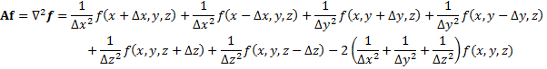
For the
calculations of the form ![]() in steps 3, 5e and 5i, we assume a 7-point
stencil and use the following finite-difference relation:
in steps 3, 5e and 5i, we assume a 7-point
stencil and use the following finite-difference relation:
|
|
|
(9) |
where
![]() ,
, ![]() and
and ![]() represent the distances to the neighbouring
grid-points in the x, y and z
directions respectively. Note that in the LEM, the grid spacing is constant in
the x
and y
directions but can vary as we move in the z direction.
represent the distances to the neighbouring
grid-points in the x, y and z
directions respectively. Note that in the LEM, the grid spacing is constant in
the x
and y
directions but can vary as we move in the z direction.
Steps 5d and 5h use a preconditioner.
The Jacobi method was chosen [11]:
|
|
|
(10)
|
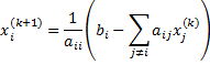
In the code,
the number of iterations of the preconditioner is set
by the parameter PREITS.
Parallel BiCGStab
For the
parallel BiCGStab, we assume the same decomposition
along the x-direction that the rest of the LEM
uses. This means that the calculations of the form of ![]() , shown in Equation 9, require
halo exchange between neighbouring processes. Steps 2, 5a, 5f, 5j and 5m
include the calculation of dot products, which require a global sum across all
the processes. Apart from these things, the other operations required by the
algorithm are local.
, shown in Equation 9, require
halo exchange between neighbouring processes. Steps 2, 5a, 5f, 5j and 5m
include the calculation of dot products, which require a global sum across all
the processes. Apart from these things, the other operations required by the
algorithm are local.
For the time
being, periodic boundary conditions have been assumed in the x
and y
directions, although alternative methods could be used. The pressure at the
boundaries in the z direction is set to zero.
The iterative
solver has been added to version 2.4 of the LEM. The following files have been
added to the source code. All the deck files contain a single procedure with
the same name as the file but without the .dk
extension. They are all subroutines apart from INNER_PROD, which is a function.
·
POISSON_ITERATIVE.dk
– solves the Poisson equation for pressure by calling the iterative solver.
This is equivalent to POISSON.dk, which uses FFTs to solve the Poisson
equation.
·
SET_MAT_A.dk
– sets the values of the matrix A such that ![]()
·
BICGSTAB.dk
– an iterative solver using the BiCGStab method.
After some experimentation, the parameters ITMAX, TOL and PREITS were set to 999, ![]() and 1, respectively. It is not expected that
the user will want to adjust them but, if necessary, their values can be
changed by editing this file.
and 1, respectively. It is not expected that
the user will want to adjust them but, if necessary, their values can be
changed by editing this file.
·
PRECOND.dk
– the Jacobi preconditioner, performing PREITS iterations.
·
CALC_Ax.dk
– calculates ![]()
·
INNER_PROD.dk
– finds the inner product of two arrays whose values are distributed across all
the processes
·
SOLVER.cdk
– a comdeck containing variables related to the
iterative solver
The following source code file, present prior to the
iterative solver, has been updated:
·
NNSTEPS.dk
– this file now contains an #ifdef-#else-#endif
structure to be resolved by the pre-processor. If the macro ITERATIVE_SOLVER is
defined then the subroutine POISSON_ITERATIVE is called; otherwise, POISSON is
called, as it is in the standard version of the LEM.
The following two files, also present in the source code
directory, have been updated to include the additional files:
·
deck.lst
– contains a list of the “decks” to be processed by nupdate.
·
comdeck.lst
– contains a list of the “comdecks” to be processed
by nupdate.
Figure 2 illustrates the relationships between the various
routines in the parallel iterative solver:
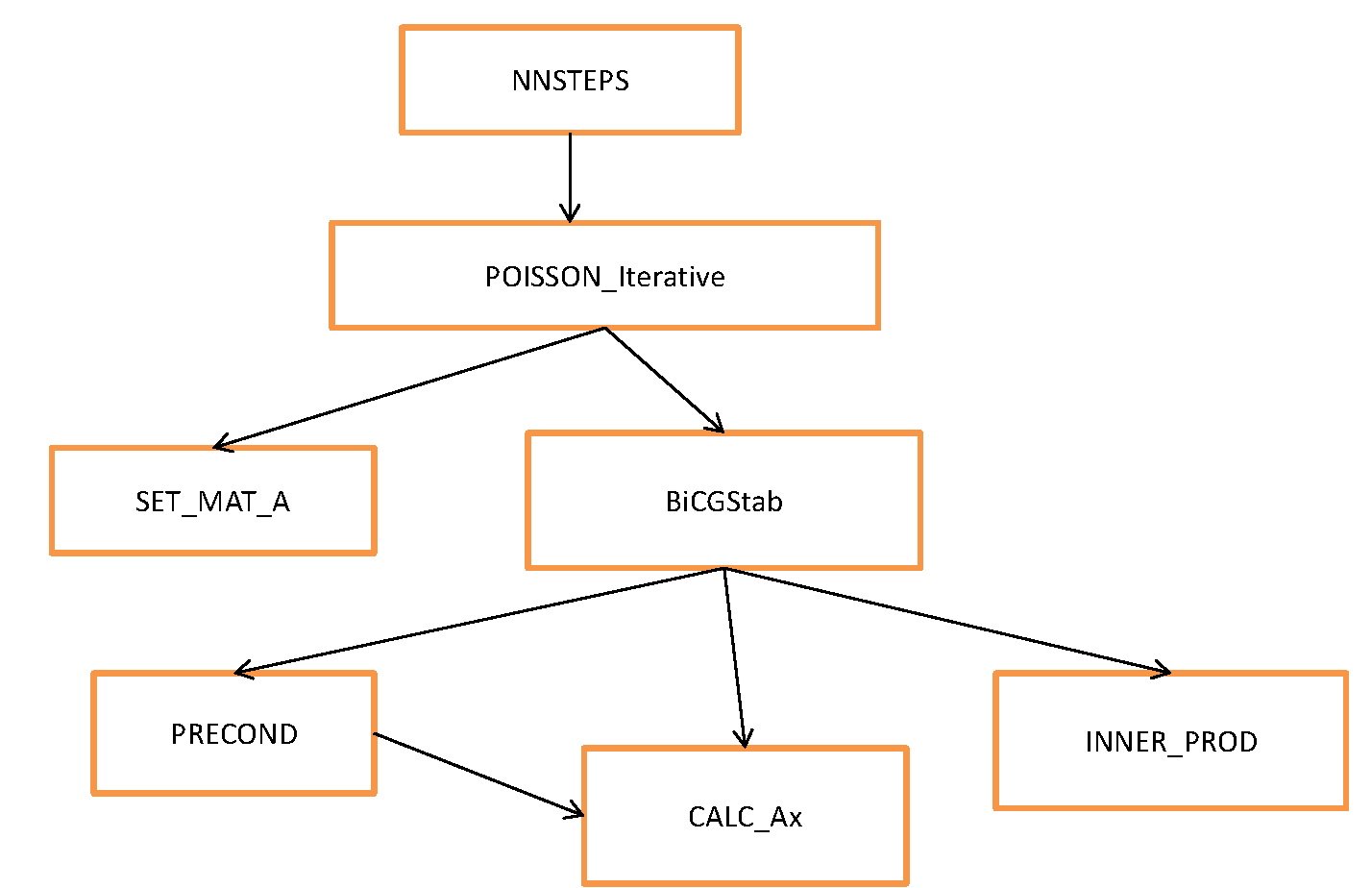
Figure 2: A call graph of the routines used
by the parallel iterative solver.
The correct operation
of the iterative solver has been verified using a test code in the following
way:
1.
Generate
a set of known pressure values, ![]()
2.
Calculate
the input source terms using ![]()
3.
Call
the iterative solver with ![]() as the input.
as the input.
4.
Check
that this gives us back our original set of pressure values, ![]()
The CrayPat profiling tool and the output from the compilers
were used to optimise the performance of the code, mainly by improving cache
re-use. The approach taken to the communication in the iterative solver is more
efficient than that used elsewhere in the code, which could really do with some
re-writing. Through profiling, it also became apparent that non-blocking
communication would give improved performance in the halo exchange. Since this
basic feature of MPI is absent from GCOM, the intermediate MPL library is
called directly where it is needed.
1.2. Code Performance
Figure 3 show
the scaling of the code with the iterative solver on phase 1 of HECToR.
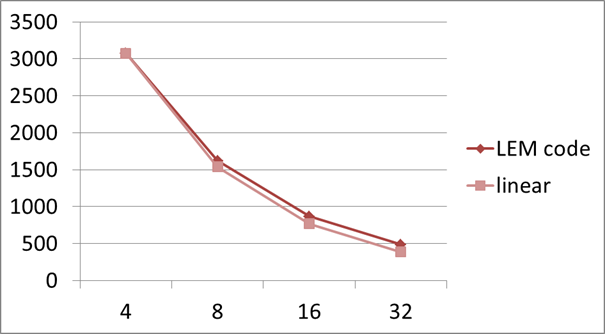
Figure 3: A graph of runtime (seconds) against number of MPI processes for the LEM code with the iterative solver on phase 1 of HECToR. Linear scaling is shown for comparison.
The code contains
two main loops. The outer one is over time and the inner one is over the set of
air parcels that move within a 1D column. This set of parcels can be divided
amongst the processes of the MPI job. There is no communication between these
parcels but their data does have to be gathered onto a single root process once
every timestep in order to output the data to a file
and to carry out the advection and sedimentation calculations. The amount of parallelism is limited by the
number of parcels in the simulation, which is often of the order of 20 to 30.
The project
successfully added an iterative solver to the Met Office LEM code. This removed
the need for periodic boundary conditions which were previously made necessary
by the use of FFTs. This enabled the code to be used in new areas of research.
The project
also parallelised the code ACPIM, again opening up new areas of investigation.
The third
goal of the project was to replace the FFT routines in the LEM code by calls to
the FFTW library. This was not carried out. This was the least important of the
objectives and it was decided to drop this due to the time needed by other
parts of the project, as well as the fact that because of the way FFTW is
licensed (GNU GPL), it would not be appropriate to incorporate these changes
into the main Met Office code.
This project
was funded under the HECToR Distributed Computational
Science and Engineering (CSE) Service operated by NAG Ltd. HECToR
- A Research Councils UK High End Computing Service - is the UK's national
supercomputing service, managed by EPSRC on behalf of the participating
Research Councils. Its mission is to support capability science and engineering
in UK academia. The HECToR supercomputers are managed
by UoE HPCx Ltd and the CSE
Support Service is provided by NAG Ltd. http://www.hector.ac.uk
[1]
http://www.hector.ac.uk/cse/
[2]
M.
E. B. Gray
and J. Petch, “Version 2.3 Of The Met Office Large
Eddy Model: Part I. User Documentation”
[3]
M.
E. B. Gray
et al, “Version 2.3 Of The Met Office Large Eddy Model: Part II. Scientific
Documentation”
[4]
M.
E. B. Gray
et al, “Version 2.3 Of The Met Office Large Eddy Model: Part III. Software
Documentation”
[5]
Jørn
Amundsen and Roar Skålin, “GC User’s Guide Release
1.1”, SINTEF Applied Mathematics, October 16, 1996.
[6]
Jørn
Amundsen and Roar Skålin, “GCG User’s Guide Release
1.1”, SINTEF Applied Mathematics, October 16, 1996.
[7]
http://www.mpi-forum.org/docs/docs.html
[8]
http://www.csm.ornl.gov/pvm/
[9]
http://staff.psc.edu/oneal/compaq/ShmemMan.pdf
[10]
Ramesh
Krishna, “Unified Model Documentation Paper X2: The Nupdate Source Code
Manager”, Met Office, November 11, 1993.