Contents
3.1 WP1: Improvement to the MPI
buffers
3.2 WP2: Efficient Memory Usage
4.1 Improvement to the MPI
Communication
4.2 Asynchronous Communication for
Complex Geometries
4.6 Compiler Performance Comparison
Enhancement
of a high-order CFD solver for many-core architecture
Lucian Anton, Ning Li and Phil Ridley,
Numerical Algorithms
Group Ltd,
Wilkinson House,
Jordan Hill Road,
Oxford, OX2 8DR, UK
August 6, 2012
Abstract
In turbomachinery
design, Reynolds averaged Navier-Stokes (RANS) models
commonly encounter problems when dealing with turbulent flows dominated by
unsteady features such as convecting wakes, large
scale separations and complex vortical structures.
These render both RANS and unsteady RANS theoretically questionable, even for
basic jets. On the other hand, Large eddy simulation
(LES) is showing tremendous promise, because the turbulent flow structures are
fully resolved numerically, rather than approximated (as in the case with
RANS). However, LES requires the use of
meshes of the order of 100 million grid points, in order to capture the intricate
turbulent flow structures. For typical simulations for fourth order space-time
correlations of turbulent fluctuations, long run times (>12hrs) are also
required. The aim of this project is to improve the performance of the structured
CFD code BOFFS, for
better use of many-core HPC architectures. The work will target the MPI
communications for the inter block transfers, achieve better memory utilisation and improve the use of OpenMP
for the intra block computations. The overall goal of the work will be to enable
realistic turnaround times for very high resolution, high-order LES by using
BOFFS with more than 100 million grid points with thousands of processing cores on
HECToR.
1
Introduction
For unsteady turbulent flows, Reynolds
averaged Navier-Stokes (RANS) models commonly
encounter problems when dealing with turbulent flows dominated by unsteady
features such as convecting wakes, large scale
separations and complex vortical structures. Examples of these are gas turbine blade
shroud flows, hub cavity/endwall regions, internal
turbine blade cooling passage flows and cutback trailing edge zones. Also, many internal air system cavity flows
are highly turbulent. These render both RANS and unsteady RANS theoretically
questionable. Even for basic jets the poor performance of RANS models is well
documented in [1][2].
On the other hand, Large
eddy simulation (LES) is showing tremendous promise. This is because the turbulent flow structures
are fully resolved numerically, rather than their effect on the mean flow being
approximated (as in the case with RANS modelling).
However, the principal difficulty in using LES is the mesh size, needed to
capture the intricate turbulent flow structures, this
is usually the order of at least 100 million grid points. This becomes especially important close to
walls where turbulent eddies are anisotropic and streak-like structures
exist. To resolve these structures
incredibly fine grids are required in the streamwise,
normal and especially spanwise directions. For the acoustic LES work performed at the
Whittle Laboratory at the University of Cambridge, fourth order space-time
correlations of turbulent fluctuations are needed. As part of assembling the spectral
information (both acoustic and turbulent) long run times are needed to
accurately resolve low frequency components, these are usually more than 12
hours. Such run-times typically involve the consumption of 5,000 kAUs per job on HECToR Phase 3.
The additional overhead of using a
general unstructured CFD solver on these scales soon becomes very apparent. Therefore an in-house
structured CFD code, namely the Block Overset Fast Flow Solver (BOFFS) has been
developed for large scale distributed parallel computations with Chimera
(overset) meshes. BOFFS is a Fortran 90 code, which uses a hybrid OpenMP / MPI approach for parallelisation.
Scalability on HECToR is reasonable for less than 10
million grid points, but it soon becomes poor for larger sized grids. For
calculations on grids of more than 100 million points, improved scalability is
necessary to be able to achieve a realistic turnaround time.
This project
will improve scalability of BOFFS on HECToR and other
many-core architectures by: optimising the MPI used
for the inter block data transfers, implementing improved memory utilisation and updating the OpenMP
for the intra block computations.
2 Code Description
The BOFFS code consists of around 22,000
lines of Fortran 90 code. This is split up into three main sections, each one
concerns a different stage in the simulation: grid pre-processing (flow
processing if restart), time advancement and solution post processing. The distributed data decomposition is such
that each grid block of the overset mesh is assigned to a single MPI process
(i.e. one block per MPI process) and within this process there is an assigned
team of OpenMP threads. Each MPI process reads in a
block of mesh coordinates, boundary condition data and if a restart is
required, the relevant flow field files will also be read. Pre-processing then consists of reading
further data and the input deck, setting boundary conditions and calculating
metric terms. In the case of a new mesh
block, interface interpolation data forms part of this stage. Once completed an interpolation file is then
written out and this will be read by any subsequent restarts. This section of the code has been
parallelised with OpenMP and is independent of the
MPI parallelisation.
Once grid pre-processing is completed, the
main time-step loop will then commence.
Here the RHS side of equations is firstly constructed. This system will
be solved using either a Gauss-Seidel or
tridiagonal matrix algorithm
(TDMA) implicit relaxation scheme – depending upon the mesh. The boundaries and
arrays will then be updated prior to the next iteration. This simple method of solution is a popular
choice for many CFD solvers since it has a low storage requirement relative to
efficiency.
When the time evolved solution has
converged, post processing will then commence.
This is straightforward and current fields are written to unformatted
binary files for restarts, and the output is also ready for Plot3D
visualisation. These output files are
written by individual MPI processes.
The most time consuming part of the code is
the transfer between block boundaries, which is required at every time step.
This involves the different physical flow variables: pressure, velocities and
temperature. Also, if turbulence modelling is used, then additional variables
are required for this exchange. The
routines which handle the transfer are PackVar_Send
and Recvvar_unpack.
Prior to this dCSE
project, some initial re-factoring of the BOFFS code was performed by NAG core
CSE and minor performance improvements were achieved. This re-factoring included:
removing unnecessary (and costly) initialisation to 0, general declarations for
undefined variables and testing the code on the range of compilers available on
HECToR. The code was also split up into manageable
.f90 files and some function in-lining performed. Use of the COMMON BLOCK was
replaced with MODULEs and a makefile was written.
3
Project Objectives
A typical 32 block case simulation could
utilise 8 fully populated 24 core HECToR phase 2b
(XE6) nodes (with 4 MPI processes per node with 6 OpenMP
threads per block) or 8 fully populated 32 core phase 3 (XE6) nodes (with 4 MPI
processes per node with 8 OpenMP threads per block).
A typical job would then take around a month in turnaround time, which equates
to around 130 kAUs and prohibits serious use of BOFFS
on HECToR.
The performance of BOFFS on phase 2b and
the comparable performance on phase 3 is given in the
following Table 1 and Table 2 for 4 test cases. Each test case has a fixed number
of grid points such that the 4BLK_3M case has 0.75 million grid points per
block, the 4BLK_12M case has 3 million grid points per block, the 32BLK_3M case
has 93,750 grid points per block and the 32BLK_12M case has 375,000 grid points
per block. Here the total timings are broken down to illustrate the time taken
to perform reading in the input data files, grid post processing and the main
time step iteration. One can see by comparing the two tables that the speed up
for the threaded code is generally quite good. But for the 4 Blocks running
over 4 MPI processes, the speedup for both 3 million and 12 million grid sizes
is good, however for the 32 Block cases the speedup is
not so good. Here the time taken for a single iteration gives only around a 2
times speed up for 6 or 8 threads.
|
Cases with OpenMP
threads |
Wall
clock time in seconds |
|||||
|
Read
Input |
Post
Processing |
1
time step |
||||
|
6
threads |
8
threads |
6
threads |
8
threads |
6
threads |
8
threads |
|
|
4BLK_3M |
1.2 |
1.0 |
1.2 |
0.9 |
30.5 |
27.1 |
|
4BLK_12M |
5.8 |
5.5 |
6.1 |
5.9 |
149.5 |
122.2 |
|
32BLK_3M |
1.3 |
1.1 |
1.9 |
1.8 |
7.5 |
5.7 |
|
32BLK_12M |
5.8 |
5.7 |
7.8 |
6.5 |
36.1 |
27.2 |
Table 1: Block
timings with 6 OpenMP threads per block on phase 2b and
8 threads on phase 3.
|
Cases with no OpenMP
threads |
Wall
clock time in seconds |
|||||
|
Read
Input |
Post
Processing |
1
time step |
||||
|
Phase
2b |
Phase
3 |
Phase
2b |
Phase
3 |
Phase
2b |
Phase
3 |
|
|
4BLK_3M |
1.4 |
1.1 |
1.4 |
1.1 |
106.7 |
82.4 |
|
4BLK_12M |
6.1 |
5.6 |
7.5 |
6.2 |
865.7 |
396.3 |
|
32BLK_3M |
1.4 |
1.3 |
1.9 |
1.7 |
34.3 |
12.63 |
|
32BLK_12M |
6.4 |
5.8 |
8.1 |
6.6 |
84.6 |
62.5 |
Table 2: Block
timings with no OpenMP on phase 2b and phase 3.
The test cases demonstrate performance for
a total number of grid points of 3 million and 12 million, with 4 and 32
blocks. All timings were produced with the GNU compiler (GCC 4.5.1 on phase 2b
and GCC 4.6.3 on phase 3). As shown in Table 1, the on node performance is good
with 6 or 8 OpenMP threads per MPI process. In Table 2, it is clear that the newer GNU
compiler (GCC 4.6.3) on phase 3 is able to perform more optimisation in BOFFS
than GCC 4.5.1 on phase 2b, and it gives better performance for the pure MPI
runs.
However, the main time step iteration does
not scale as expected for larger problem sizes. Output from automatic profiling
analysis shown in Figure 1, implies that the routine for packing the MPI buffer
across blocks in a synchronous manner (PackVar_Send)
is a problem. Further analysis in Figure 2 shows that there is a significant
load balance problem caused here too, which in turn increases the MPI
synchronisation times.
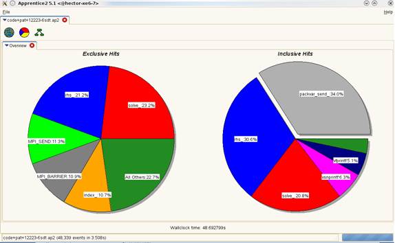
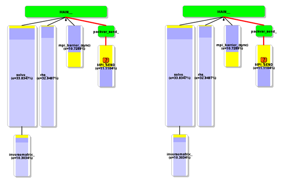
Figure
1: Automatic profiling analysis of a 3 million grid point, 32 block case. Figure
2: a) Load imbalance for PackVar_Send and b) Call graph (3
million grid point, 32 block case).
In addition to the scalability problem,
during core CSE investigation, it was discovered that BOFFS generally performed
better with the PGI compiler (version 10.9.0) rather than the GNU one – due to
improved optimisation in the areas of loop unrolling and vectorisation.
However, this was only investigated using the smaller (3 million) grid point
case, for larger problem sizes, the use of large static arrays for all
variables within BOFFS caused out of memory errors. Furthermore the use of OpenMP scheduling was not optimal within the intra block
computations. The following work was therefore proposed for this project:
3.1 WP1: Improvement to the MPI
buffers
WP1.1 Within the MPI packing/unpacking
routines: PackVar_Send and Recvvar_unpack,
the double precision buffer Var_Recv_Mpi stores the
data (boundary values of pressure, velocities and turbulence equation
quantities) which are needed at every time step. The packing and unpacking of
this buffer uses five levels of nested IF...THEN loops within the three level
DO loops (below).
E.g.
do k = Nk1, Nk2
do j = Nj1, Nj2
zn_num =
zonenumber(nblock,1,j,k)
do z = 1, zn_num
zn_type =
zonetype(nblock,z,1,j,k)
if (zn_type .ze. 0) then
bnd1 =
zoneboundm(nblock,z,1,j,k)
bnd2 =
zoneboundp(nblock,z,1,j,k)
if (bnd1.eq.b_int)
then
if ((val .Eq. 0).or.(val .Eq. b_int)) then
block = nbb(nblock,z,1,j,k)
if (block.eq.from_block) then
count =
count + 1
PbndM(nblock,z,1,j,k) = Var_Recv_Mpi(count)
This will be upgraded so that the data
structures can be aligned beforehand in a way that the IF…THENs may then be
removed. Pre-determined off-sets will be used for count rather than
incrementing. This will be achieved by
implementing the following approach:
nblock = rank
do np = 1, npbound
i = mpi_index(np)
j
= mpi_index (np+1)
k = mpi_index (np+2)
z = mpi_index
(np+3)
count = countindex(np+4)
PbndM(nblock,z,1,j,k) = Var_Recv_Mpi(count)
enddo
Here the mpi_index array will be calculated as part of the
pre-processing phase, and incorporated into the interpolation file. Using this approach it will be possible to
move from five levels of nested IF...THEN loops within the three level DO loops
to a single do loop which should significantly boost performance.
WP1.2 The rest of the work needed to
improvement the performance of the inter block transfers will be to replace the
existing (serial) MPI communication scheme with an asychronous
method, so that there is a significant reduction in synchronisation time. This
will be achieved by mixing computation with communication, and therefore
replacing the existing communication pattern of the point to point
communications which use a left to right serial transfer. The combined effort
of WP1 is expected to give at least a representative 20% speedup in performance
and enable good scalability up to at least 100 blocks (1000+ cores).
3.2 WP2: Efficient Memory Usage
Large static arrays are used for all
variables including those for the interface, primitives (steady and unsteady), RHS,
boundary, and output metrics. For the 12 million grid point cases, these are
too large for the PGI compiler with mcmodel=medium,
however, they work fine with dynamic linking. They also work fine as static
arrays for the GNU compiler. But for the
3 million grid point case, the PGI compiler is 10% faster than GNU and it would
therefore be beneficial for performance to get BOFFS working with PGI for all
problem sizes without the need for dynamic linking. This will be achieved by
replacing all necessary static arrays with allocatable
ones and removing any redundant arrays where not required.
3.3 WP3: Validation
All
work will be validated on the 32 and 4 block test cases, both with 12 million
grid points.
4 Project
Outcomes
4.1 Improvement to the MPI Communication
In order to improve the MPI buffers, a further analysis of BOFFS was
performed. Before any development to the PackVar_Send and Recvvar_unpack routines was performed, the method of calling
these transfer algorithms was updated. Originally, a serial method of calling
the MPI communications was used to exchange data between blocks. Here, each MPI
process would perform a loop over the total number of MPI tasks with a blocking
receive waiting for the previous process to send the data. The following
example which uses 5 MPI tasks for simplicity, illustrates the situation:
Considering 5 MPI tasks, with each task
passing a data buffer to the left neighbour the communication pattern is
0 <- 1 <- 2 <- 3 <- 4
with
call mpi_send(sbuff,...,myid-1...,ierr)
.....
call mpi_recv(rbuff,...,myid+1,..,ierr)
Here every rank posts a blocking send to
the left first, but only rank 0 can proceed to the receive call (for
non-periodic boundary conditions). Then after the exchange (0 <- 1)
completes, rank 1 will move to receive the call and then the (1 <- 2)
exchange can progress and so on. But this is serialised communication which
could be completed in just two parallel operations.
In terms of the effects on code
performance, the following profile by function group and function, shows that
for the 12 million 32 block test case, 9.3% of the run time is taken up in MPI,
in particular most of this time is consumed by the blocking MPI_SEND routine.
Time% |
Time | Imb. | Imb. | Calls |Group
100.0% | 230.205369 | -- |
-- | 14281280.8 |Total
|-------------------------------------------------------------------------------------------
| 82.3% | 189.357545 | -- |
-- | 14280789.6 |USER
||------------------------------------------------------------------------------------------
|| 38.6% | 88.894237 |
2.648718 | 3.0% | 40.0 |solve_.LOOP@li.212
|| 12.8% | 29.496465 |
2.303737 | 7.5% | 1.0 |main_
||
9.8% |
22.588643 | 0.093898
| 0.4% | 42.0 |rhs_.LOOP@li.223
||
9.3% |
21.451923 | 0.090482
| 0.4% | 42.0 |rhs_.LOOP@li.1812
||
7.5% |
17.350544 | 0.079816
| 0.5% | 42.0 |rhs_.LOOP@li.1024
||
2.4% | 5.448789 | 2.663316 | 33.9% | 14280000.0 |inversematrix_
||
0.9% | 2.102017 | 0.009066 | 0.4% |
42.0 |rhs_
||
0.5% | 1.058167 | 0.028250 | 2.7% |
61.0 |boundaryupdate_.LOOP@li.144
||
0.3% | 0.692370 | 0.003452 | 0.5% |
40.0 |solve_
||
0.1% | 0.126090 | 1.943039 | 96.9% |
3.8 |boundaryupdate_.LOOP@li.479
||
0.1% | 0.117772 | 0.003597 | 3.1% |
61.0 |boundaryupdate_.LOOP@li.1182
||=================================================================
|
9.3% |
21.368852 | --
| -- | 112.4 |MPI
||------------------------------------------------------------------------------------------
||
7.7% |
17.813062 | 18.727963 |
52.9% | 40.7 |MPI_SEND
||
1.1% | 2.603411 | 1.503864 | 37.8% |
1.0 |mpi_finalize
||
0.4% | 0.951937 | 0.112093 | 10.9% |
40.7 |mpi_recv
||
0.0% | 0.000376 | 0.000128 | 26.2% |
21.0 |MPI_BARRIER
||
0.0% | 0.000051 | 0.000007 | 12.6% |
6.0 |mpi_wtime
||
0.0% | 0.000006 | 0.000001 | 9.2% |
1.0 |MPI_INIT
||
0.0% | 0.000005 | 0.000001 | 23.2% |
1.0 |mpi_comm_rank
||
0.0% | 0.000004 | 0.000001 | 24.6% |
1.0 |MPI_COMM_SIZE
||=================================================================
| 8.5% | 19.474334 | 19.223893 | 98.7% |
21.0 |MPI_SYNC
||------------------------------------------------------------------------------------------
|
8.5% |
19.474334 | 19.223893 |
98.7% | 21.0 | mpi_barrier_(sync)
||=================================================================
By applying a simple trick (where firstly
the odd ranks post their receives and then the even
ones post their sends), the packing subroutine will drop out from the
statistics. With this method, the communication is done in parallel between
distinct pairs in two stages:
Stage 1: (0 <- 1), (2 <- 3) , 4
Stage 2: 0, (1 <- 2), (3 <- 4)
code pattern
if (
mod(myid,2)==0)then
call mpi_recv(rbuff,...,myid+1,..,ierr)
...
call mpi_send(sbuff,...,myid-1...,ierr)
else
call mpi_send(sbuff,...,myid-1...,ierr)
...
call mpi_recv(rbuff,...,myid+1,..,ierr)
endif
In terms of the effects on code
performance, the following profile by function group and function, shows that
for the 12 million 32 block test case, now only 3.1% of the run time is taken
up in MPI, in particular less than 1% of the time is consumed by the blocking
MPI_SEND routine. For this test case, the overall speed gain is that the
MPI_SEND time drops from ~18 seconds to 1.8 seconds which gives an overall run
time decrease from 230 to 203 seconds.
Time% |
Time | Imb. | Imb. | Calls |Group
100.0% | 203.165181 | -- |
-- | 14281280.8 |Total
|------------------------------------------------------------------------------------------
| 93.2% | 189.367336 | -- |
-- | 14280789.6 |USER
||-----------------------------------------------------------------------------------------
|| 43.8% | 89.040701 | 3.005270 | 3.4% |
40.0 |solve_.LOOP@li.212
|| 14.7% | 29.898026 | 4.079582 | 12.4% |
1.0 |main_
|| 11.2% | 22.674467 | 0.095291 | 0.4% |
42.0 |rhs_.LOOP@li.223
|| 10.4% | 21.225894 | 0.077735 | 0.4% |
42.0 |rhs_.LOOP@li.1812
||
8.6% |
17.393574 | 0.079199 | 0.5%
| 42.0 |rhs_.LOOP@li.1024
||
2.5% | 5.018218 | 2.621076 | 35.4% | 14280000.0
| inversematrix_
||
1.0% | 2.098218 | 0.008748
| 0.4% | 42.0 |rhs_
||
0.5% | 1.061462 | 0.028729
| 2.7% | 61.0 |boundaryupdate_.LOOP@li.144
||
0.3% | 0.679213 | 0.002862
| 0.4% | 40.0 |solve_
||
0.1% | 0.127722 | 1.979859 | 97.0% | 3.8 |boundaryupdate_.LOOP@li.479
||
0.1% | 0.119386 | 0.003574
| 3.0% | 61.0 |boundaryupdate_.LOOP@li.1182
||=================================================================
|
3.7% | 7.496753 | 6.046087 | 80.6% | 21.0 |MPI_SYNC
||-----------------------------------------------------------------------------------------
|
3.7% | 7.496753 | 6.046087 | 80.6% | 21.0 | mpi_barrier_(sync)
||=================================================================
|
3.1% | 6.296505 | -- |
-- | 112.4 |MPI
||-----------------------------------------------------------------------------------------
||
1.4% | 2.920704 | 1.907597 | 40.8% | 1.0 |mpi_finalize
||
0.9% | 1.827206 | 2.685173 | 61.4% | 40.7 |MPI_SEND
||
0.8% | 1.548190 | 0.217016 | 12.7% | 40.7 |mpi_recv
||
0.0% | 0.000340 | 0.000057 | 14.8% | 21.0 |MPI_BARRIER
||
0.0% | 0.000051 | 0.000005
| 9.2% | 6.0 |mpi_wtime
||
0.0% | 0.000006 | 0.000002 | 29.7% | 1.0 |MPI_INIT
||
0.0% | 0.000005 | 0.000008 | 65.4% | 1.0 |mpi_comm_rank
||
0.0% | 0.000005 | 0.000004 | 44.5% | 1.0 |MPI_COMM_SIZE
||=================================================================
After
this development, the PackVar_Send and Recvvar_unpack routines do not show up in the profile and
therefore, there would not be any useful performance gain by improving the
loops in the original plan for WP1, since the time spent in those packing loops
is a very small fraction of the total run time.
4.2 Asynchronous Communication
for Complex Geometries
After updating the MPI communication with an odd / even
MPI_SEND and MPI_RECV transfer, it was noticed that the existing communication
method limited the scope of BOFFS to grids where individual blocks were related
to either one or two neighbouring blocks. In practice, this is restrictive
because in a typical mesh there may be a central core block that all outer
blocks must interface with e.g. for a compressor blade or jet mesh simulation.
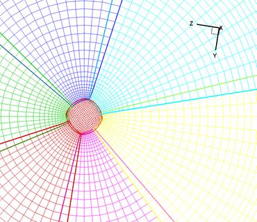
Figure 3: Example of a jet mesh.
However, the situation was improved by implementing
asynchronous communication in the form of MPI_ISEND, MPI_IRECV and MPI_WAIT.
This was achieved by storing the number of neighbouring blocks for each
individual block (MPI task), then pre-posting the MPI_IRECVs before the calls
to PackVar_Send and the
MPI_ISENDs. Now the buffers are loaded and each MPI process will be ready and
waiting to receive incoming data from its’ neighbours.
Although, each task still has to wait, this is a very short time for grids
where each block has an even distribution of neighbours. Overall, this improves
the performance of the communications as well as enabling grids with more
complex block structures. This method of communication also gives a further 1%
improvement over the odd / even MPI_SEND and MPI_RECV transfer.
4.3 Efficient Memory Usage
The original BOFFS used large static arrays
for all main variables including those for the interface, primitives (steady
and unsteady), RHS, boundary, and output metrics. These are all contained
within the file arrays.mod which defines the MODULE arrays. Approximately 100
static arrays contained within this module were subsequently updated to allocatable form. The introduction of allocatable
arrays also makes the code more flexible as the array dimension can now be read
from an input file, hence there is no need to recompile
the BOFFS code when changing the array sizes for different grids.
For the 12 million grid point cases, these
now work with the PGI compiler thus enabling at least a 10% representative
speedup over the GNU compiler.
4.4 Updating the OpenMP
In addition to the original objectives, a short
study was done for the scalability of the OpenMP
sections in solve.f90. This routine performs the TDMA solver and from the
previous CrayPAT profile, it can be seen that it
takes up 43.8% of the overall run-time, in particular the main loop. With the
initial OpenMP implementation scalability was lost
above 6 threads, because the local domain was very narrow in one direction
(i.e. on average 40:1).
To improve OpenMP
scalability, a red-black decomposition of computation was implemented in
solve.f90 for the main loop and this algorithm now scales reasonably up to 32
threads. In addition to the
implementation of the red-black decomposition for the OpenMP
threads, the number of OpenMP threads available is
now collected with the omp_get_max_threads function
which gets the number straight from the OMP_NUM_THREADS environment variable.
While testing scalability with the default compilers
on HECToR, it was noticed that PGI was having a
problem running the code with more than a single thread, even though it worked
fine with GCC and CCE. The code would not progress past the main loop in solve.f90 and it was discovered that this was due to the
volatile use of an INTEGER array, 'map'. The solution was to use the following
declaration of ‘map’
INTEGER, volatile ::
map(0:maxsizeline,0:maxsizeline)
The directive !$OMP FLUSH(map) was already in the
code, but volatile variables are part of the Fortran 2003 language standard,
both GCC and CCE were able to identify this whereas PGI was not.
Furthermore the source code was split as one module per
file for a faster compilation and some out of bound array accesses were
corrected. The NAG compiler was also used (in depend mode) to generate makefile dependencies for the new BOFFS source code.
4.5 Validation
To
validate the updated version of BOFFS, several runs were performed on phase 3.
These were done to both check the results and record timings for the new code. All
runs were performed using code compiled with GCC 4.6.3, as this was used to
compile the original version of the code. The runs were performed with 1, 2 and
4 MPI tasks per 32 core HECToR phase 3 node. A
comparison between the original and new code is given in Table 3. Here, we see
that for the new code scalability is only better for the 32BLK_12M and 32BLK_3M
cases, this is because these both involve more MPI communication than the 4BLK
cases. In the case of the single threaded runs, the new code is slower for the
4BLK cases due to the overhead with the creation of the new OpenMP
implementation for the main TDMA solver. However, there is a 1.4 times speedup
in the 32BLK cases due to the improved OpenMP in the
TDMA.
|
Test
Cases |
Wall clock time
to perform 1 time step (in seconds) |
|||||
|
Original code |
New code |
|||||
|
1 thread |
8 threads |
1 thread |
8 threads |
16 threads |
32 threads |
|
|
4BLK_3M |
82.4 |
27.1 |
114.5 |
30.5 |
26.3 |
25.4 |
|
4BLK_12M |
396.3 |
122.2 |
544.15 |
137.4 |
122.0 |
115.0 |
|
32BLK_3M |
12.63 |
5.7 |
16.4 |
4.0 |
4.0 |
4.6 |
|
32BLK_12M |
62.5 |
27.2 |
62.8 |
18.5 |
18.1 |
18.5 |
Table 3: Comparison
between the original and new code.
4.6 Compiler Performance
Comparison
Before
the beginning of this project, it was noticed that BOFFS gave better
performance with PGI than with GCC, so the aim of WP2 was to enable the code to
compile with PGI. Therefore, results will be presented for the performance of
the new BOFFS code with the default compilers on HECToR:
Gnu (GCC), PGI and Cray (CCE).
The
compiler options (FLAGS) which give the best code performance for BOFFS are as
follows:
GCC
4.6.3 FLAGS= -Ofast –fopenmp
PGI
12.5.0 FLAGS= -fast –mp
CCE
8.0.6 FLAGS= -O ipa1
The
results in Figures 4-7 show that CCE generally gives best performance and OpenMP scalability, with PGI a close second.
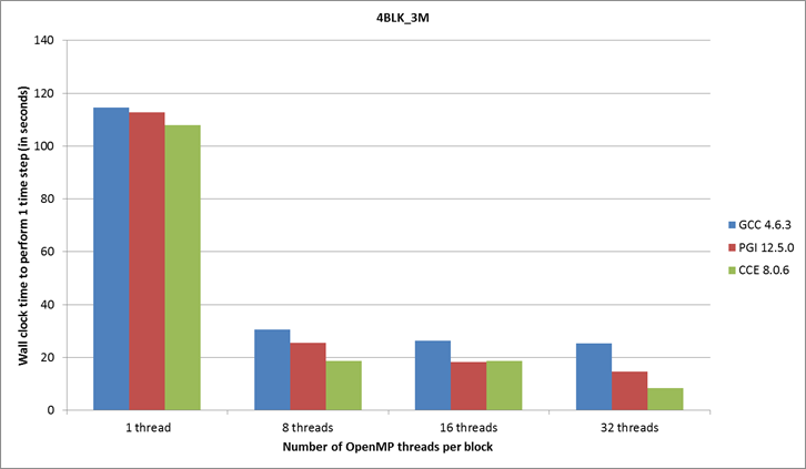
Figure 4: Compiler performance for the 3 million grid point, 4 block
case.
Scalability
of the OpenMP is better for the 4BLK_3M and 4BLK_12M test
cases as shown in Figures 4 and 5, this is due to the larger number of grid
points per block (i.e. 750,000 and 3 million) and so there is more scope to get
a good speed up going from 8 to 32 threads per block. Scalability for up
to 8 OpenMP threads is efficient for all four of
these test cases, however use on only problem sizes comparable the larger
4BLK_3M and 4BLK_12M cases may prove worthwhile.
All
runs were performed with at most one MPI task per 8 core NUMA die and in the
case of the 4BLK_12M test case, each MPI task was allocated to a single Interlagos 16-core chip due to the larger memory
requirements (i.e. the phase 3 nodes used were half populated).
For
the 4BLK_12M and 32BLK_12M test case results shown in Figures 5 and 7, the new code with PGI
or CCE gives on average a 1.5 times speedup for the 12 million grid point, 4
and 32 block cases, which is better than the original aim of achieving a 20%
speedup.
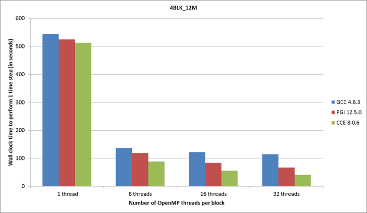
Figure 5: Compiler performance for the 12 million
grid point, 4 block case.
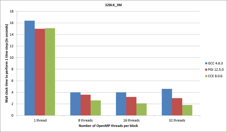
Figure 6: Compiler performance for the 3 million
grid point, 32 block case.
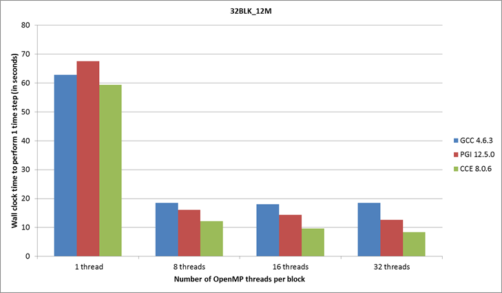
Figure 7: Compiler performance for the 12 million
grid point, 32 block case.
In general, the most cost
effective solution for using BOFFS on HECToR phase 3
is with 8 OpenMP threads, and either 2 or 4 MPI tasks
per node depending on the size of the problem.
5 Example
Simulations
To end this report, some recent results from LES and hybrid RANS-NLES
simulations performed with BOFFS on HECToR, will be
presented:
5.1 High Pressure Turbine
This is an instantaneous flow from a BOFFS
calculation of a high pressure turbine blade (HPT) as given in Figure 8 showing
zones of separated large scale vortical structures
contaminating the span of the blade.
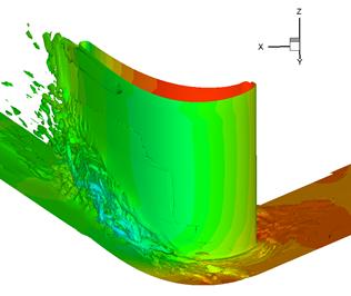
Figure 8: Flow in
high pressure turbine using RANS-NLES.
5.2
Low Pressure Turbine
BOFFS simulations of a flat
plate with an imposed pressure gradient, representative of a low pressure
turbine blade (LPT), are presented. The upper
boundary of the computational domain is specifically contoured to impose an
adverse streamwise pressure gradient as shown in
Figure 9.
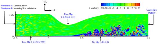
Figure 9: Computational domain and the boundary
conditions considered. Contours show z-vorticity, with incoming box turbulence.
This is representative of the
flow around the leading edge of a LPT blade. Two simulations, without and with
incoming free-stream turbulence, labelled Simulation A and B respectively were
also performed. The incoming turbulence
intensity was set to 4% in simulation B.
|
(a) |
(b) |
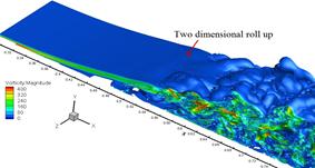
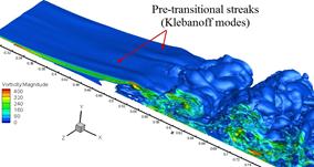
Figure 10: Iso-surfaces of vorticity magnitude for: (a) Simulation A with laminar
inflow, (b) Simulation B with turbulent inflow.
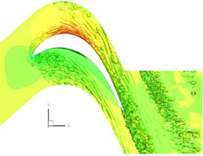
Figure 11: Wake induced
transition and end wall flow for a T106A blade.
The iso-surfaces
of vorticity magnitude for simulations A and B are
shown in Figure 11. While the separated shear layer prior
to transition is fairly two dimensional in simulation A, spanwise
undulations clearly appear in simulation B. These undulations are the
footprints of what are called Klebanoff modes. A
successful eddy resolving approach needs to capture such modes when modelling
LPTs.
5.3 Rim Seal
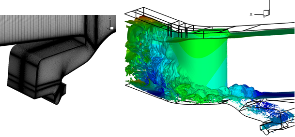
(a) (b)
Figure 12: (a)
Cavity LES grid, (b) vorticity magnitude isosurfaces for cavity geometry.
Using BOFFS with a validated modelling methodology
the interaction of sealant flows with the main stream can be studied in much
greater depth. An example is given in
Figure 12(b) where the rim seal cavity flow can be seen to substantially
influence the main passage endwall and separation
zones. The use of LES and hybrid RANS-NLES will allow many more complex flow
systems to be studied in detail and improved upon, at a cost much lower than
that of experimental rig testing.
5.4 Labyrinth Seal
A labyrinth seal geometry as shown in
Figure 13 is representative of those found at blade tips/shrouds and throughout
the internal air system. The flow
generated by this seal is again complex.
It includes regions of high acceleration, separation, recirculations of different scales and a high velocity rotating
lower wall.
In Figure 13 (a), vorticity
contours of the flow field are shown. There is high vorticity
near the rotating wall showing the boundary layer type flow, with vortices shed
off the tooth tips. Hence this flow
contains both wake and boundary layer type turbulence.
All of the simulations presented can be
obtained in less than 1 month using 500 processing cores.
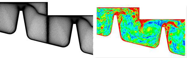
Figure 13: (a) Lab
Seal Mesh, (b) Vorticity magnitude contours of Lab
Seal LES flow field.
6
Conclusions
The aim of this project was to enable at
least a representative 20% speedup in performance over the original BOFFS code
and also enable scalability to at least 100 blocks. The results in section 4
have demonstrated that this has been achieved and OpenMP
scalability has been improved in general, for up to 8 threads. In particular
the new code with PGI or CCE gives on average 1.5 times speedup for the 12
million grid point, 4 and 32 block case. Furthermore, using the 12 million grid
case with 4 blocks as an example having 3 million grid points per block,
comparative weak scalability for a problem just over 30 times larger would take
BOFFS to more than 100 million grid points and more than 100 blocks.
Given that BOFFS is a versatile overset, structured code, it will
continue to be used on HECToR for a variety of turbomachinery problems including heat and cooling film
technology. It will also provide a
platform for broadband noise calculations that will require of the order of
4,000 kAUs per HECToR
job. Immediate plans include
collaborating with other members of Cambridge UGTP Whole Engine Computational Aeroacoustics Consortium, who have successfully obtained an
EPSRC grant for computing resources on HECToR. In particular, this dCSE
work will now allow BOFFS to use HECToR to facilitate
the development and testing of new ideas which have been generated from
previous research. It is also planned to
collaborate with internationally leading research groups and the wider HPC
community through the next UK Applied Aerodynamics HECToR
consortium. Through
EP/I017771/1, the UKTC and the new UKAAC (under
preparation) substantial resource (15,000 kAUs)
is planned for allocating to BOFFS usage for investigation of the aerodynamics
and aeroacoustics of complex geometry hot jets.
7
Acknowledgements
This project was funded under the HECToR
Distributed Computational Science and Engineering (CSE) Service operated by NAG
Ltd. HECToR A Research Councils UK High End Computing
Service - is the UK’s national supercomputing service, managed by EPSRC on
behalf of the participating Research Councils. Its mission is to support
capability science and engineering in UK academia. The HECToR
supercomputers are managed by UoE HPCx
Ltd and the CSE Support Service is provided by NAG Ltd. http://www.hector.ac.uk.
The authors would also like to thank the main developer of BOFFS, Dr Richard Jefferson-Loveday of
the Department of Engineering at the University of Cambridge, for ongoing
discussion and also for providing the results shown in Figures 8-13.
8 References
[1] Georgiardis, N.
& DeBonis, J., 2006, “Navier
Stokes Analysis Methods for Turbulent Jet Flows with Application to Aircraft
Exhaust Nozzles”. Progress in
Aerospace Sciences., Vol. 42, pp. 377-418
[2] Secundov A. N., Birch S. F. and Tucker P. G. 2007, “Propulsive Jets and their Acoustics”, Philosophical Transactions of the Royal
Society (Series A: Mathematical, Physical and Engineering Sciences) Vol.
365, pp.
2443-2467.