
Abstract
Tensor Network Theory (TNT) provides efficient and highly accurate algorithms for the simulation of strongly correlated quantum systems. The corresponding numerical algorithms enable approximate descriptions of many-body states and linear operators acting on them that do not grow exponentially with system size, in contrast to exact descriptions. Whilst TNT algorithms are efficient, they are numerically demanding and require high-performance optimised and parallelised implementations. A TNT library is currently being developed at the University of Oxford to allow users to have access to the complex algorithms needed to solve these problems from their own high level codes.
This project is concerned with optimising and parallelising those parts of the TNT library that involve heavy computations, to enable important quantum effects in many-body systems to be studied. The initial objectives were:
Contents
The TNT library is a numerical software suite for researchers investigating tensor network theory for quantum interactions. It has been developed by Prof Dieter Jacksch’s group in the Physics department at the University of Oxford. Based originally on a series of Matlab scripts it has now grown into a full library, developed in C. This library is now being used by a rapidly growing number of other researchers outside its original group through its release via the CCPForge repository [1]. Therefore all developmental work on increasing the performance of the software will be very useful to a broad range of researchers using these algorithms. This meant that minimising the changes to end-users’ codes was imperative, despite the inclusion of parallelism using MPI and OpenMP in this project.
The cases that users are simulating using this software are varied, however there are particular algorithms that are very commonly applied. The work done in this project is fully tested around the most common of these, the time-evolving block decimation (TEBD) algorithm. The main operations in the TNT software typically involve combinations of matrix-matrix multiplications, singular value decompositions (SVD) and matrix rearrangements. The standard TEBD algorithm, for example, at each node of the 1-d network, involves three contractions (which are a rearrangement and a matrix-matrix multiply) and one SVD. A brief overview of this algorithm is given in the next section.
In brief, the aims of this dCSE project were to help optimise the TNT library for all users and to include the parallelism necessary to facilitate the solution of large matrix problems and large networks. The three objectives listed in the Abstract were split between two work packages. The first work package was more focused on the basic performance of the code (Obj. 1 & Obj. 2), with a second work package on using the sparse matrix structure that exists in many cases to achieve improved performance (Obj. 3). Parallelism is also included in both of these topics.
In the sections to follow the work done is split into three parts. In Section 3 the optimisations made to the code for serial and OpenMP execution are discussed in relation to each of the three objectives. The introduction of MPI parallelism into the partitioning of the network, which aids in both Obj. 1 and Obj. 2, and the necessary changes to the algorithms used, are described in Section 4 along with its parallel scaling. In Section 5 an additional layer of MPI parallelism is outlined for use with very large matrices, which forms an important part of Obj. 3.
The library defaults to making use of the standard linear algebra routines provided in LAPACK. Where applicable these both are accelerated through the use of multithreaded MKL or, on HECToR, ACML or LibSci. These vendor libraries already use OpenMP and hence even the initial version of the software had significant parallel performance enhancements through the use of increasing numbers of threads. The parallel work here, thus, had to augment these capabilities.
As the work progressed a minor change was made to the original workplan. In Obj. 3 it had been envisaged that the MPI parallelism would be employed within individual SVDs to distribute the blocks formed between processors. The improvements made in working on Obj. 1, Obj. 2, and the serial version of Obj. 3 showed that typically using OpenMP to distribute the work between the available cores was suitably efficient. As such the MPI parallelism is deployed at the network level with separate operations able to be efficiently computed concurrently resulting in significant performance gains. This is all explained in Section 4. In order to closely satisfy this objective the capability for extremely large matrices to be split using MPI has also been developed; see Section 5.
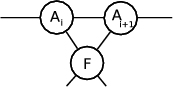
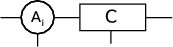
In this work only one-dimensional tensor networks are considered. These may be represented schematically as shown here:
Each circle, Ai, represents a separate site in the network, with legs being the lines joining the sites together. Every site has a tensor with a set of indices of size χ. Larger χ values give more accurate results, although obviously at the cost of extra computation. The physical legs have dimension d, which was 2 in the systems studied here, but can vary depend on the system being studied.
Numerical methods based on TNT are well established in the scientific community. The first key breakthrough was the density matrix renormalisation group (DMRG) algorithm for studying static system properties, developed in 1992. As an indication of its significance, as part of its 50th anniversary, Physical Review Letters nominated the original proposal [2] a ‘Milestone Letter’ of 1992. The corresponding breakthrough for the simulation of coherent dynamics was in 2003-04 [3] with the time evolving block decimation algorithm (TEBD). A number of variants and enhancements of these original algorithms has been developed over the following years [4] which have been highly successful at obtaining novel insights into the physics of strongly correlated quantum systems [5].
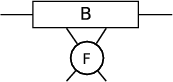
The standard TEBD algorithm works by performing a sweep across the network from one end to the other, followed by a sweep in the reverse direction. The algorithm works by considering pairs of sites, performing operations on them, then moving the pair under consideration one site further right. For two neighbouring sites, Ai and Ai+1, first a ‘unitary’ node, F , is attached to them both. Then the two neighbouring A sites are contracted together, before being contracted with the unitary:
→ |
→ |
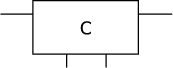
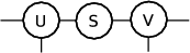
with an SVD being performed on the result to leave new tensors U, S and V :
→ |
→ |
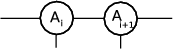
where U becomes the new Ai. S and V are then contracted to form the new Ai+1. At this point the algorithm moves to the next pair, Ai+1 and Ai+2.
Of particular note for the parallelism in this project is the serial nature of this algorithm. It is only possible to update Ai+2 once the updates of Ai and Ai+1 have both completed.
For the systems considered in this work it is typical that χ is small (set to 2) for the sites at the ends of the network.
Each successive site then has a doubling in size up to the maximum value, χmax, which is typically constant across most
of the length of the network. This does mean that many operations will be done on large systems, however there will
always be cases of small dimensions at the ends of the networks which will have some impact on the performance of the
individual algorithms applied in the library. For instance, if the boundary site has a 2×8 matrix structure, as in the
examples that follow, then a χmax of 200 would not reach the maximum size until the eighth site along,
meaning 40% of the network would be solving smaller systems than in the middle. For χmax=600 then
half the sites are working on computationally much cheaper systems since the algorithms applied are
typically  (n3). For all systems with open boundary conditions, with physical dimension d, the internal
dimension D increases by a factor of d for each internal bond from the boundary up to a maximum value of
χmax.
(n3). For all systems with open boundary conditions, with physical dimension d, the internal
dimension D increases by a factor of d for each internal bond from the boundary up to a maximum value of
χmax.
The goals of the first work package were to “optimise tensor storage and improve SVD, contract and reshape operations”. The target speed-up for this work, Obj. 1 and Obj. 2 was a 20% improvement in run-time. The application of OpenMP was included in this expected performance increase. For the second work package, blocking the matrices for the SVD and the matrix-matrix multiply, Obj. 3, a 20 times speed-up was expected.
In this section the improvements to the serial and OpenMP implementations of each of the main components of the code is discussed in detail, highlighting which of the objectives the work fitted into. First, the reshape operation is discussed in 3.1, followed by the SVD in Sections 3.2 and 3.3, and finally the contract operations in Section 3.4 and 3.5. Results for the overall speed-ups from doing this work are explained clearly in Section 3.6.
The work which was undertaken was primarily based on code profiling undertaken on the original software base with the costliest functions targeted. These were, as expected, the reshape, the SVD and the matrix multiply. In fact over 99% of the run-time is spent in these three sections.
All timings in this section are run on the TNT group’s target cluster at the University of Oxford. This is a combination of 20 Quad-Core Dual processor Dell 64-bit Xeon Harpertown 2.0 G Hz cores and 36 Quad-Core Dual processor Viglen Xeon Nahelem 2.2 G Hz nodes cores, with all timings done on the faster nodes. More results from other machines are given later in the Section 4. The Intel compiler and the NAG and MKL libraries have been used for all results generated in this section. The test case chosen is ten timesteps of the TEBD algorithm at sizes χmax=150, 300 and 600.
In the original code the reshape operations took roughly 10% of the time of the (unmodified) SVD or the matrix-matrix multiply. A major difference between the reshape and the other two, though, was that there was no OpenMP in by default compared to the highly tuned MKL versions of D/ZGESVD and D/ZGEMM. This meant that when the number of threads was increased, the reshape time was not affected, thus the reshape could end up more costly than the others. By adding OpenMP to the reshape function this has successfully enabled scaling with increasing numbers of threads.
The reshape operation is a way of mapping the indices of a tensor with multiple legs (i.e. dimensions) into new locations in a two-dimensional matrix. It is therefore a computation involving only integers. This transformation is obviously dependent on the dimension of the supplied matrix and is unique up to permutations of the dimension of the legs of this tensor. Cases typically have hundreds or thousands of timesteps and would therefore be performing identical reshapes (of different matrices) many times. The number of repeated calculations is increased further by realising that through the majority of the network the sites have an identical tensor dimension of χ=χmax meaning that the transforms performed on one of these sites will be repeated on the others.
In order to reduce this computational overhead a method for reusing the calculated reshapes has been implemented. Every time a new combination of leg dimensions is encountered, new memory is allocated for the storage of the remapping of the matrix entries. When a case that has already been seen is needed the correct reshape translation is simply retrieved from memory. In cases where the value of χmax changes it may be necessary to free some of this storage if no longer needed. Similarly in cases with large numbers of reshapes the memory requirements for storage would be too great, then reshape reuse may be disabled, either permanently or just for sections of the execution.
In practice this change has made a huge difference to the performance of the reshape operation. Whilst the cost of the initial calculation cannot be avoided (although work done on minimising the operation count of this section has speeded that part alone up 20%) the reuse is extremely efficient. An example is shown in Table 1 which gives the reshape timings for both the original and final versions of the code.
| Original | Enhanced reshape
| |||
| χmax | Threads | No reuse – 10 steps | Reuse storage (once) | Reuse – 10 steps |
| 150 | 1 | 6.3 | 0.09 | 0.7 |
| 2 | 3.5 | 0.06 | 0.7 | |
| 4 | 2.0 | 0.04 | 0.7 | |
| 8 | 2.1 | 0.04 | 0.7 | |
| 300 | 1 | 25.3 | 0.43 | 3.8 |
| 2 | 14.1 | 0.25 | 3.1 | |
| 4 | 8.3 | 0.17 | 2.9 | |
| 8 | 7.5 | 0.29 | 3.4 | |
| 600 | 1 | 93.4 | 1.87 | 15.5 |
| 2 | 53.8 | 1.14 | 13.6 | |
| 4 | 31.6 | 0.69 | 12.4 | |
| 8 | 24.6 | 0.47 | 12.7 | |
The column labelled “Original” includes the work on both the operation count reduction and adding OpenMP. It can be seen how without the reshape reuse the scaling with the number of OpenMP threads is excellent. If reuse is enabled, of the 3622 calls to the reshape function for the χmax=600 case, only 132 are in the initial setup period thus resulting in new translations being calculated and hence stored. This means that only a small percentage of the total runtime is calculating these mappings. This part, as shown in Table 1, scales well using OpenMP. When reusing this information the cost is fixed for as long as the matrix sizes stay fixed, hence the other 3490 calls just retrieve matrix locations from memory meaning a fixed cost per cycle for the reshapes is found. For example on four threads the cost per iteration is reduced from 3.16s to 1.24s. The performance on other size matrices is similar with smaller matrices allowing higher cache reuse, and bigger matrices enabling better OpenMP scaling.
Overall:
∙ A 20% improvement was seen in the cost of the reshape by minimising the operation count.
∙ Excellent OpenMP scaling is seen for the calculation of new reshape data.
∙ A total speed up factor of 5–10 times is seen using the memory reuse.
∙ The limiting factor is the memory bandwidth, hence why minimal advantage is seen on these problem sizes with more OpenMP threads.
The computation of an SVD at every site in the network on every timestep is the highest cost involved in these calculations. This is especially true given how the matrix-matrix multiply scales better using OpenMP and the optimisation work done in vendor LAPACK implementations. As such improving the performance of the SVD was identified as very important.
The first area of focus was looking at the matrices being decomposed, and in particular the values they contained. It was seen that they often contained a lot of numbers close to zero, including subnormal numbers. Since all the vectors making up the matrix are normalised that means that the small values are making negligible contributions to the computed singular values and their associated vectors.
The use of a (user definable) tolerance parameter, TOL, was therefore added to the software. At the start of the SVD, all matrix entries smaller than TOL were set to be zero. Similarly, all small entries in the calculated U and V matrices were also set to zero. Where the calculated singular values themselves were less than TOL the associated vectors were changed to zeroes with a one on the diagonal (an identity vector for this singular value). By adding this functionality it ensured that all small values calculated during the SVD in areas that should have been identically zero, remained zero, thus preserving any sparsity structure that should have existed analytically. It also ensures that this numerical noise that develops during the SVD does not get the opportunity to grow and pollute the computed results.
With so many zeroes being inserted into the matrices there are often entire rows and columns of zeroes. This is
especially the case in the early stages of a simulation or after a change in χmax. These zero rows and columns can
therefore be safely removed from the calculation of the singular values as they correspond to calculating a
singular value of zero. As before these are subsequently chosen to have identity vectors added to the U
and V matrices. The reduction in size of these matrices is therefore significant as the SVD algorithm is
 .
.
In all the work done in this project the introduction of TOL is the only change made that affects the results calculated in the code. There are a few particular cases where the choice of this parameter is very important as using the subnormal numbers can give slightly more accurate answers. However the extra computational cost involved in not using it, especially when combined with the blocking work that follows in Section 3.3, makes not using it very unattractive.
The performance of the improved SVD is shown in Section 3.3, however it is worthwhile to note the affect of TOL on the accuracy of the results computed. Comparisons of many cases, with different values of TOL (including negative to disable the functionality) have been analysed. The results show that, as expected, the tolerance chosen for setting values to zero in the SVD converges as it gets smaller. A value of TOL = 1×10⁻⁸ can be taken as too large, but TOL = 1×10-12 has been accurate for all cases tested. This is obviously important as it gives users an extra control on accuracy versus computational cost. Note the use of TOL also avoids the growth of errors from parts of the matrices which should remain zero.
In the project work plan it was noted how symmetry information about the physical systems could often be used to accelerate the execution of the codes by reducing the most costly parts to operating only on smaller dense blocks. These were, namely, the SVD, the matrix-matrix multiply and the reshape. Following the zeroing work done in the previous section the rearrangement of the matrix had already been set up for the removal of the zero rows and columns. That code could also then be deployed to rearrange the non-zero rows and columns as desired.
An example state of a matrix for the SVD is shown in Figure 1a
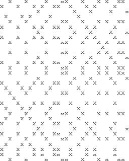
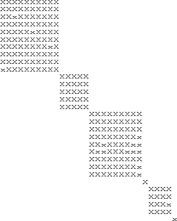
(a) Unordered (b) Reordered
which shows a small matrix which had previously been passed to the SVD after the removal of the zero rows and columns. Whilst no overall structure is obvious from this picture it is possible to rearrange the rows and columns to get the image shown in Figure 1b. In this case a single supposedly ‘dense’ block has been rearranged to six smaller blocks, two of which are just single values.
The overall algorithm for producing the blocked structure from just the matrix is outlined in Algorithm 1. Each of the steps in this algorithm is listed with the size of the matrices in question at the end.
The algorithm for the rearrangement part (step 3, including the removal of the zero rows and columns (step 2) is given in Algorithm 2.
This involves three loops over the matrix. The first effectively “pushes rows up” to get, for example, all the rows with entries in the first column at the top; the second pushes the columns left. These two loops alone form an almost completely blocked structure, however in certain cases it is necessary to push rows up once more to guarantee the blocked structure. Note that the second two of these loops necessitates non-sequential memory access, harming performance through significant numbers of cache misses on large matrices. These effects are reduced by constructing of a look-up array, with one byte per element denoting if the entry is below or above TOL. This means that the cost of multiple absolute value tests is avoided, and the array is 8 (or 16 for complex cases) times smaller in memory.
Once the rearranged matrix has been formed individual blocks can be extracted on which the SVD can be solved independently of the other blocks, (step 7 in Algorithm 1). Typically this is done using a multithreaded LAPACK implementation, such as MKL. In practice the OpenMP parallel region has been extended further out than just the SVD to enable the pre- and post-processing of that block (steps 6 and 8) to be done in parallel. For efficiency reasons parallelisation of these parts are only done provided the total matrix to be decomposed, dimension Mnnz×Nnnz, is sufficiently large.
A difference between using the single block method and this multiblock approach is in the size of matrices that are returned from the SVD. When the matrix is treated as a single block the system solved is:
where K = MIN(M,N). It is the sizes of U, S and V that are changed in the multiblocked case such that Uis [M×M] and Vis [N×N]. The extra rows or columns returned will not affect the final result as they correspond to singular values of zero, however the implementation of the reinsertion of the output back into the matrices in step 8 is significantly simplified.
The LAPACK implementation returns the singular values in decreasing order, hence when the full matrix is solved in a blockwise fashion each separate block will have its singular values organised thus. Therefore it is necessary to reorder the U, S and V matrices to give the singular values in S in the expected order (step 10).
Note that if the entire system is a single block then the intermediate steps translating the matrix to secondary arrays can be avoided, and the SVD can return the desired final sized matrices by default.
The advantages of this approach to the solving of the SVD on a multicore system are twofold. Most importantly the
size of the matrix which is being decomposed is often significantly reduced. As noted above, the SVD has  complexity, hence reducing the size of the systems being solved is computationally very beneficial. Also it has been
seen how the SVD itself does not scale perfectly with increasing numbers of OpenMP threads, especially for small
systems. Therefore applying the parallelism higher up at the block level seems to allow more useful computation to be
performed concurrently.
complexity, hence reducing the size of the systems being solved is computationally very beneficial. Also it has been
seen how the SVD itself does not scale perfectly with increasing numbers of OpenMP threads, especially for small
systems. Therefore applying the parallelism higher up at the block level seems to allow more useful computation to be
performed concurrently.
To demonstrate the effectiveness of the blockwise approach timings are given in Table 2 for the same three test cases described in Section 3.1.
| Original | Enhanced SVD
| ||||
| χmax | Threads | No blocking | No Blocking | Blocking enabled | Blocking |
| No TOL | TOL=1×10-12 | TOL=1×10-12 | overhead | ||
| 150 | 1 | 84.1 | 23.2 | 3.5 | 1.6 |
| 2 | 56.6 | 17.7 | 1.9 | 1.2 | |
| 4 | 41.5 | 13.5 | 1.7 | 1.0 | |
| 8 | 39.1 | 12.4 | 1.9 | 1.0 | |
| 300 | 1 | 592.4 | 269.2 | 28.9 | 9.6 |
| 2 | 351.3 | 170.0 | 15.3 | 7.0 | |
| 4 | 224.2 | 113.0 | 12.0 | 5.8 | |
| 8 | 215.1 | 107.0 | 14.2 | 5.8 | |
| 600 | 1 | 4007.6 | 2022.0 | 164.2 | 34.8 |
| 2 | 2267.3 | 1207.9 | 85.3 | 26.7 | |
| 4 | 1423.0 | 788.7 | 72.1 | 22.5 | |
| 8 | 1252.8 | 726.8 | 79.9 | 22.9 | |
Here the reduction in computational time through using the TOL value (column 4), described in Section 3.2, can be clearly seen when compared to not using it (column 3). Typically this is reducing the computational time for the SVD between 2 and 4 times. Note that the blocking work could not happen without the use of TOL since the numerically calculated SVD would have had small, non-zero entries in the areas of the matrix which should be zero due to physical symmetries. The enabling of blocking on top of this gives an overall reduction of between and 10 and 20 times, even including the overhead in manipulating the matrices before and after computing the SVDs on the blocks.
Overall:
∙ The use of TOL gives a reduction in computational time of a factor of 2–3.
∙ A total speed up of 10–20 times is seen using the blocked SVD on problems up to χmax=600. Larger problems or having more blocks perform even better.
∙ OpenMP scaling of the SVD is enhanced by doing not just the SVDs of individual blocks in independent threads, but also having the preparation and post processing for those blocks similarly distributed.
∙ The overhead costs of blocking the matrix are due to non-uniform memory access, harming cache reuse, again being limited by memory bandwidth, hence why minimal advantage is seen on these problem sizes with more OpenMP threads.
The TEBD algorithm described in Section 2 describes the system at each sitewise pair being solved using a single SVD (step (4)) sandwiched between three contractions, steps (2), (3) and (5). Each contract necessitates a tensor reshape to change the dimensions of the matrix representing the tensor to have the correct dimensions for the matrix-matrix multiply which combines the two tensors together.
Of the three contractions shown, the first is multiplying two dense matrices together, the second involves one dense and one unitary matrix, and the third involves one dense and one diagonal matrix. Up to this point this diagonal S matrix had always been stored in the library as a dense matrix with the inefficiency of this single matrix-matrix multiply being masked by other expensive calculations. However it will be seen in Section 4 how an alternative TEBD algorithm, denoted here pTEBD, can have many more operations involving diagonal matrices per site update. Specifically this algorithm will have seven contractions, five of which involve a diagonal matrix plus one with the unitary, leaving only a single dense-dense multiply. In addition it will also involve two matrix inverse calculations.
The cost of a matrix-matrix multiply, for matrices sized [M×N] and [N×P] is normally  . For a diagonal
second matrix, for example, this cost can be reduced to
. For a diagonal
second matrix, for example, this cost can be reduced to  . In addition, the unitary matrix, F in TEBD steps (1)
and (2), can be very small since it has size d4, where d is the physical dimension of the system. In the cases in this
report d = 2 meaning the matrix-matrix multiply operation involving it is effectively
. In addition, the unitary matrix, F in TEBD steps (1)
and (2), can be very small since it has size d4, where d is the physical dimension of the system. In the cases in this
report d = 2 meaning the matrix-matrix multiply operation involving it is effectively  . Note that the largest case
done in this work is multiplying matrices [2χmax×χmax]×[χmax×2χmax], and the unitary multiply is
[χmax2×d2]×[d2×d2].
. Note that the largest case
done in this work is multiplying matrices [2χmax×χmax]×[χmax×2χmax], and the unitary multiply is
[χmax2×d2]×[d2×d2].
The matrix inverse operation is even more inefficient when treating the matrix as dense. It actually just requires
taking the reciprocal of the individual diagonal elements, hence is an  computation rather than
  , where S is
[N×N].
, where S is
[N×N].
The timing results for these changes are demonstrated in the next section, where it is seen that the matrix-matrix
multiply is speeded up by a factor of between  and
and  and the matrix inverse has become a negligible cost in the
pTEBD algorithm. These are the expected values given the total number of dense multiplies no longer being
computed.
and the matrix inverse has become a negligible cost in the
pTEBD algorithm. These are the expected values given the total number of dense multiplies no longer being
computed.
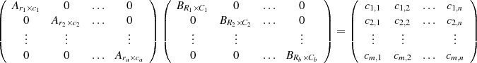
Similar to the SVD the matrix-matrix multiply is done on matrices which frequently contain many zeroes, with a similar, potentially blocked structure. As such, performing the expensive matrix-matrix multiply operation on these unmodified is overly wasteful of resources. The main differences this time to the SVD are that there are two matrices which need reshaping into blocked form, and that the output is a single matrix, which also has a blocked form.
The matrix-matrix multiply operation on matrices A and B is given by:

By rearranging A into blocked form (as shown previously in Figure 1) there is already a restriction placed on the reordering of B. Namely, that is the rows of B must be permuted as the columns of A were. This obviously includes that any columns removed from A which are identically zero must have the corresponding row removed from B. Note that this does similarly set up a feedback condition that any zero rows in B should have the corresponding column of A removed. Once A has been reordered the columns of B can be permuted to give the final block structure. Since this blocking typically corresponds to a physical property of the system being solved and have come from the blocked SVD, it is likely that these blocks coincide well.
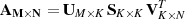
Since the block structure of A and B are not guaranteed to be identical a composite structure is formed. For example if A is divided into a blocks of dimension ri ×ci and B into b blocks of dimension Ri ×Ci, as in:
then an extra block dividing line should be made whenever the blocking of columns of A does not match that of B. An example of this is A and B, each size 4N ×4N both being made of two blocks, but with distinct boundaries. If we consider each block in A to be 2N ×2N and the blocks of B to be 3N ×N and N ×3N, one gets:
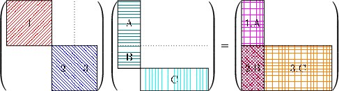
Computationally the structure of the final C matrix is found by performing a matrix-matrix multiply on a tiny system just containing the structure of each of these matrices, with the output being which input blocks are needed to find the answer. For the system above that would be:
where the output matrix, C, has non-zeroes in  =
=  ths of the matrix, however the calculation cost is
reduced from (64N3) to (10N3). Such a reduction should easily compensate for the overhead costs of
rearranging the matrices, all of which will be (n2) but with significant amounts of random memory
access leading to poor cacheline reuse. Real cases have many more blocks than this illustrative example,
hence the time spent in calculating the Z/DGEMM calls will be significantly smaller. This does mean,
however, that the blocking cost is about five times the size of the cost of the resulting (smaller) Z/DGEMM
calls.
ths of the matrix, however the calculation cost is
reduced from (64N3) to (10N3). Such a reduction should easily compensate for the overhead costs of
rearranging the matrices, all of which will be (n2) but with significant amounts of random memory
access leading to poor cacheline reuse. Real cases have many more blocks than this illustrative example,
hence the time spent in calculating the Z/DGEMM calls will be significantly smaller. This does mean,
however, that the blocking cost is about five times the size of the cost of the resulting (smaller) Z/DGEMM
calls.
One of the other side-effects of this is that the parallel efficiency of the matrix multiply is seemingly diminished. However it is important to note that the matrix size being solved is now significantly smaller. Typically for the test cases here there are an average of five or six structural blocks being solved and hence, because the OpenMP scaling is only visible on larger cases, there is no longer a speed-up with increasing numbers of threads for the matrix-matrix multiply seen at these problem sizes.
Timings for the increase in performance of the matrix-matrix multiply are given in Table 3 where the same test cases as in Sections 3.1 and 3.3 are used. Also shown in Table 3 are the equivalent timings for running the alternative TEBD described in the next section, denoted here as pTEBD, showing timings for both the matrix-matrix multiply and the matrix inverse calculations. Comparing the two sets of results, denoted “Dense MM” and “Diag. MM”, for both algorithms clearly shows that, irregardless of problem size or the number of threads used, the use of the diagonal matrices whenever possible reduces the total cost by about a third for the TEBD and two thirds for the pTEBD. This obviously correlates extremely well with the number of dense matrix-matrix multiplies no longer being performed.
| Original | Final | Original | Final | Original | Final | |||
| TEBD | pTEBD
| |||||||
| Threads | Dense | Diag. MM | Blkd MM | Dense MM | Diag. MM | Blkd MM | Dense Inv | Diag. Inv |
| χmax = 150 | ||||||||
| 1 | 11.0 | 7.6 | 2.2 | 2.4 | 0.8 | 0.5 | 0.5 | <0.1 |
| 2 | 5.8 | 4.0 | 2.2 | 1.3 | 0.5 | 0.6 | 0.4 | <0.1 |
| 4 | 3.3 | 2.3 | 2.0 | 0.8 | 0.3 | 0.6 | 0.4 | <0.1 |
| 8 | 2.2 | 1.9 | 2.0 | 0.8 | 0.3 | 0.6 | 0.3 | <0.1 |
| χmax = 300 | ||||||||
| 1 | 79.0 | 53.3 | 14.5 | 61.5 | 17.8 | 6.0 | 10.2 | 0.2 |
| 2 | 40.3 | 27.4 | 11.1 | 31.8 | 9.8 | 5.9 | 6.2 | 0.1 |
| 4 | 21.3 | 14.9 | 9.9 | 16.9 | 5.9 | 5.7 | 4.0 | 0.1 |
| 8 | 19.3 | 13.9 | 10.5 | 13.4 | 5.7 | 5.9 | 3.7 | 0.1 |
| χmax = 600 | ||||||||
| 1 | 562.9 | 375.8 | 58.1 | 226.8 | 64.5 | 15.6 | 35.2 | 0.8 |
| 2 | 286.8 | 191.7 | 44.8 | 116.4 | 34.6 | 14.9 | 20.2 | 0.4 |
| 4 | 149.3 | 101.4 | 41.4 | 61.1 | 19.8 | 14.4 | 11.8 | 0.3 |
| 8 | 122.5 | 89.6 | 42.7 | 45.0 | 20.7 | 14.8 | 10.2 | 0.2 |
Note that these timings include treating all matrices as dense on their first encounter after loading.
The lines marked “Blkd MM” show the speed-up from using the blocked versions of these routines. The results show that the blocking has similar performance improvements to the equivalent work on the SVDs. As expected these cases are only efficient for many OpenMP threads at large χmax due to the relatively high serial overhead of the reshaping operations. Overall, though, on large matrices the serial performance, even including this overhead, is four to six times better than the non-blocked, but diagonalised time.
Overall:
∙ A total speed up of up to 20 times is seen using the blocked form over the original.
∙ The time for the matrix inverse has been effectively removed entirely.
∙ The limiting factor is the memory bandwidth, hence why minimal advantage is seen on these problem sizes with more OpenMP threads.
In this section all the major optimisations that have been included in the TNT library software have been explained in detail. In short these have been built around exploiting the sparsity structures that typically exist in the matrices being exhibited at every stage, or reusing information that could have been saved from previous calculations. These have all provided at least the predicted performance increases in satisfying Obj. 1, Obj. 2 and Obj. 3.
An example of the final performance of these aspects of the code is shown in Figure 2.
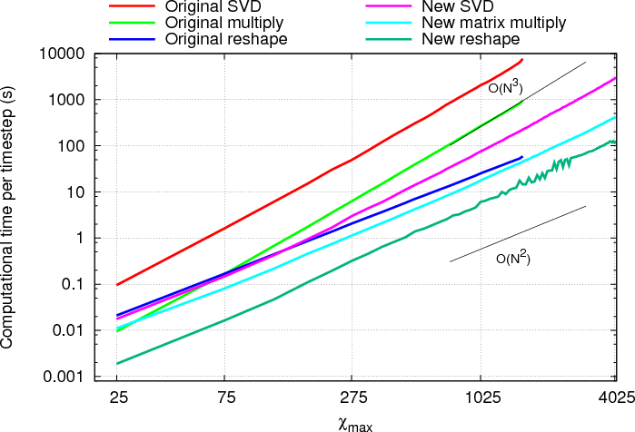
This graph shows the computational time taken for each of the three main components of the software, namely the
SVD, the matrix-matrix multiply and the reshape. Note that the blocking costs for the matrix-matrix multiply and the
diagonal-dense multiplies are already included in that total. Guide lines have also been added to indicate (N2) and
(N3) performance.
The results show that the fully optimised code performs significantly better than the original code. The SVD is clearly the most expensive part in the final code, but this performs over 30 times better than the original at large matrix sizes. It must be stressed that this increase is directly attributable to the use of the tolerance enabling the blocking to take place; without it the SVD would still be performed on a single dense block, hence performing similarly. The matrix-matrix multiply is similarly improved, but most notably the growth of this section is dominated by the blocking work before and after, hence the algorithm scales better to bigger problem sizes than that of the original method. Additionally the reduced number of dense-dense calculations being made increases performance.
The small variations in performance of the reshape for χmax between 1400 and 2000 is directly attributable to the test case chosen. This case has a rapid growth in the entanglement meaning that χmax is increases quickly. In this period the number of steps between increasing is either 1, 2 or 3 thus limiting the reshape reuse that can be made. The difference in performance is thus very noticeable here, but small compared to the additional costs involved in increasing χmax by larger amounts but less frequently.
The standard TEBD algorithm that forms the heart of many tensor network theory simulations is inherently serial, as explained in Section 2. This is due to the dependency on completing the update on site Ai before moving to Ai+1, with this being true all the way across the network. When considering the current scaling of the software and the potential speed-ups that may be achievable, alongside the desire to move to large systems in two space dimensions, it was clear that simply adding more parallelism into the operations described above would not produce a scalable solution. Instead the parallelism needed to be applied at the tensor network level which would necessitate finding an alternative to the standard sweeps of the TEBD.
The solution to this problem is to use an alternative TEBD that is termed here the pTEBD algorithm [3, 6]. This uses an even-odd style of update where the network can be considered to be made up of alternating even sites and odd sites. Updates are made pairwise, similar to before, but all pairs starting on even sites are updated on one timestep with all odd sites updated the next. The updates made on one pair are independent of all the others meaning that this algorithm is inherently parallel.
The initial state for the pTEBD algorithm is different to that shown in Section 2. Here as well as the main sites, denoted Γi, there are intermediate sites λi, which contain only a diagonal matrix of the singular values formed during an SVD.

In order to update site Γi it is necessary to consider Γi, Γi+1, λi-1, λi and λi+1
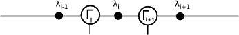
and first add copies of λi-1 and λi+1 with their inverses into the network:
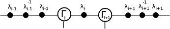
The unitary node, F , may then be joined to the two Γ nodes
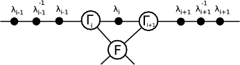
before contractions join λi-1 to, Γi, to λi, to Γi+1, to λi+1 then finally to the unitary
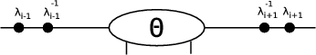
to give a node, Θ. This system is then split using an SVD to give nodes U, S and V . U is then contracted with λi-1-1 and V with λi+1-1:
with the results designated the new Γi and Γi+1. This algorithm has thus calculated new nodes Γi, Γi+1 and λi.
This may seem a more demanding algorithm, with seven contractions and two inverses required. However, as was noted above in Section 3.4, the fact that the λi are diagonal matrices means that the contractions and inverses are very cheap to calculate. In fact there are five dense:diagonal, one dense:unitary and only one dense:dense multiply. In addition it transpires that the matrices formed during the update are actually smaller than the equivalent cases in the standard TEBD algorithm. This is due to using a different singular value truncation tolerance which explains the significant drop in times for the matrix-matrix multiply seen in Table 3. The same tolerance could, equally, be applied in the TEBD case.
Note that using the pTEBD algorithm there is only a single update of each site in the network per timestep, unlike the standard TEBD which sweeps one way then the other. However the pTEBD does require timesteps to be half the size of those for the standard TEBD algorithm in order to give comparable Trotter errors [7]. The results are thus independent of which algorithm is chosen.
In order to solve networks with large numbers of sites or with very large tensors stored at the sites it was necessary to develop a distributed memory version of the TNT library. The pTEBD algorithm enables the execution of the network itself to be executed concurrently and the storage of the network to be fully distributed.
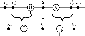
In order to spread the network across a series of computational resources (hosts) the sites in the network are initially partitioned between the hosts in a straightforward manner of attempting to share the number equally. Each host loads a full copy of the network connectivity, however only the host that ‘owns’ a site loads the tensor information and this is the significant memory usage. A simple example is to consider dividing a small network between two hosts:
where p0 and p1 are the two processors. The labelled sites are the ones owned by that processor. Note in this case λ3 is owned by both processors.
With this partition it is possible to apply the pairwise pTEBD update. In order to perform an update on a pair of Γ sites it is necessary to have Γi, Γi+1, λi-1, λi and λi+1 present on the same host. Communication of the data stored on sites is thus necessary between hosts. For the simple partition explained above this is as follows.
For the ‘even’ update site Γ1 is uninvolved, p0 can work on the pair Γ2-Γ3 and p1 on Γ4-Γ5. Note that in this case all the processors have all the λi values they need to update the nodes they need, and that it is only the even λi that are changed so no communication is necessary as λ3 is unchanged by the updates taking place on either side of it.
Applying the ‘odd’ update in this case does require communication. The chosen convention in the code is to perform the computation on the left hand host of any pair of Γi-Γi+1 sites meaning in this simple case p0 is computing the pairs Γ1-Γ2 and Γ3-Γ4, whereas p1 is idle as Γ5 is uninvolved. Communicating Γ4 and λ4 from p1 to p0 is necessary before the update of Γ3-Γ4 can take place. Once it is complete λ3 and Γ4 need communicating back to p1.
For actual simulations there are typically many sites per processor. In fact there is never any advantage in having more processors partitioning the network than half the number of sites since some would always be idle, either during the even or odd update. In fact it is best to have multiple pairs to be updated per host since that way computation of pairs inside a host’s partition can be completed whilst non-blocking communication of the sites needed for the first and last sites on that partition are completed. This use of non-blocking communication was found during the development to be essential for efficient parallelism as it allows significant out-of-order execution of the pairwise updates.
The communication of the data on sites in the network is not trivial. Computationally sites are actually a nest of structures containing many variable length arrays. In order to communicate this efficiently between processors the relevant data size is first calculated by the owning processor then all that data is all put into a single continuous MPI_PACKED buffer. The use of non-blocking communications necessitates the size of the message be known before an MPI_Irecv call is posted as the receiving buffer must have been allocated beforehand. Since this would remove any possibility for overlap of these communications the use of MPI_Iprobe to check for the arrival of a message (with the expected tag) and the size of that message meant that this buffer need only be allocated upon delivery, and then processed using MPI_Recv.
The partitioning of the network that is done at load time is based purely on equidistributing the number of sites between the available hosts. For many cases, such as those used in this report, this is not ideal as the sites towards the boundaries of the network have much smaller sizes, hence the amount of computational work needed on these sites is far less than those in the middle of the network. Similarly if run on a heterogeneous architecture with processors of different speeds, such as run by the TNT group, then this will also lead to significant load imbalance. Therefore dynamic network repartitioning has been implemented. Periodically, say every ten timesteps, the software looks at the computational time taken to compute the network update on each host. These times are then collected and a new partition formed. Nodes are sent to their new host in exactly the same way as during an update, however this time the representation of the network on each host is also ‘cleaned’ to free memory from nodes that are no longer resident there.
It is important to note that none of the parallelism added to the library during the distribution of the network, or using the pTEBD algorithm interferes with the OpenMP acceleration exhibited by the underlying routines. This means that all the same speed-ups for the SVD, matrix-matrix multiply and the reshape will still be present. In fact the only part of Section 3 that changes the performance of the MPI parallelisation is the diagonalisation of the λi sites, meaning that the cost of communicating them is significantly cheaper.
The scaling of the parallelised TNT library is explored in this section. Summarised below are representative results from two different test cases that have been run on two separate resources. The important differences between the cases that are of relevance to the parallel scaling are how the value of χmax grows over the simulation and the total number of sites in the network. The larger χmax values mean that the individual computations are more significant, ensuring better OpenMP scaling, as evidenced in the previous section. The number of sites is important since the larger this is, the more processors may be effectively used in partitioning the network.
The computational timings presented here have been run on two separate machines. The first is the Arcus cluster at the University of Oxford which is made up of 84 16-core nodes running 2.2GHz Xeon SandyBridge with 64GB RAM per node. The second is the UK’s national supercomputing resource, HECToR, which has been used in its Phase 3 configuration, which is a Cray XE6 system with 2816 nodes each containing a dual processor 16-core AMD Opteron 2.3GHz Interlagos and 32GB RAM. Note that on HECToR only every other core is used since adjacent cores share a single floating-point unit which significantly impacts upon the calculation time of the SVD and the matrix-matrix multiply.
Results are shown in Table 4 for these cases.
|
|
|
|
|
|
|
|
Number of threads
|
|||||
| Procs | 1 | 2 | 4 | 8 | 16 |
| 1 | 1.00 | 1.48 | 1.89 | 1.92 | 1.88 |
| 2 | 1.84 | 2.71 | 3.16 | 3.25 | - |
| 4 | 3.18 | 4.17 | 4.78 | - | - |
| 8 | 4.22 | 5.62 | - | - | - |
| 16 | 5.82 | - | - | - | - |
| Number of threads | |||
| Procs | 1 | 2 | 4 |
| 1 | 1.00 | 1.58 | 1.87 |
| 2 | 1.87 | 2.97 | 3.44 |
| 4 | 3.41 | 5.41 | 6.18 |
| 8 | 5.03 | 7.50 | 5.52 |
| 16 | 7.79 | 10.30 | 12.78 |
| Number of threads | |||||
| Procs | 1 | 2 | 4 | 8 | 16 |
| 1 | 1.00 | 1.64 | 2.19 | 2.18 | 2.11 |
| 2 | 1.88 | 3.04 | 3.70 | 3.62 | - |
| 4 | 2.93 | 4.81 | 5.33 | - | - |
| 8 | 4.19 | 6.01 | - | - | - |
| 16 | 4.42 | - | - | - | - |
| Number of threads | |||
| Procs | 1 | 2 | 4 |
| 1 | 1.00 | 1.72 | 1.75 |
| 2 | 1.89 | 3.25 | 3.32 |
| 4 | 3.33 | 5.72 | 5.78 |
| 8 | 4.68 | 6.21 | 5.60 |
| 16 | 5.16 | 7.44 | 9.18 |
This gives the total solution time for the runs as described, and hence the overheads of the poor OpenMP performance of the initial small matrices is included in the total times given.
It can be seen how increasing the number of MPI processes, i.e. having more partitions, always improves performance. This is most evident for Case 1 with 100 sites where each processor has more sites on which to work per timestep. Increasing the number of threads up to 4 is always beneficial, too, but on the problem sizes tested no benefit was seen beyond this number. The most interesting part of these tables is considering the best way to deploy an available resource. This can be seen by looking diagonally north-east, to compare identical core counts. For the large number of sites case it is almost always best to use the available cores on partitioning the network whereas for the other case using two threads is beneficial beyond two processors.
The performance difference between Arcus and HECToR is noticeable. Since the CPUs have similar clock-speeds the major difference is thus the choice of LAPACK implementation, with ACML seeming to perform at half the speed of MKL. Use of LibSci rather than ACML gave similar scalings. Whilst slower overall, HECToR does provide better parallel scaling.
Simulations of the networks performed in this work have been limited to one dimensional cases. Rather than simulating two dimensional cases on full 2-d networks which would require a more complicated algorithm it is possible to reduce them to a one dimensional case, albeit with very large matrices at each site.
It has been seen how the network can have the sites successfully split across a network of processors using MPI and that on each of these resources that OpenMP parallelism within the resource can be used within the LAPACK calls. In order to better distribute the work for large matrices one of the objectives of this work was to investigate splitting the SVD over multiple MPI processes.
An investigation of MPI versions of SVDs was conducted on HECToR. One important limit on the choice of library providing this functionality was that a large number (χmax) of the (χmax×d) singular values, and their corresponding vectors, of the matrices are required rather than just the few largest or smallest. This limited range is offered very efficiently by packages such as SLEPc or ARPACK but is not useful for the users of the TNT software. As such, the choice for finding all singular values and vectors was therefore ScaLAPACK, Elemental and libFLAME.
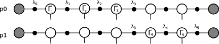
A series of cases investigating the parallel performance of the SVD compared to the baseline of the optimised threaded ACML LAPACK code was tested on randomly generated dense complex matrices at a range of sizes up to 10 000×10 000 using up to 96 processes on HECToR, i.e. three full nodes. An example graph showing the relative performance of these three libraries is shown in Figure 3
for a fixed height of 6000 rows, but varying the number of columns. The results all suggest that the fastest SVD is achieved through using libFLAME and Elemental together. Althogh not shown here, ScaLAPACK appears to scale better than either option using Elemental, however it seems to start from a much higher baseline. It was notable during the development that the coding overhead of using libFLAME and Elemental was significantly smaller than that of using ScaLAPACK. One drawback, though, is that since these libraries are still being actively developed there is some functionality still to be completed.
By choosing to substitute the SVD operation for one from ScaLAPACK or libFLAME/Elemental it was also important to ensure that the performance of the matrix-matrix multiply was not adversely affected. Without reproducing any of those results here, it was seen that ScaLAPACK and Elemental had broadly similar performance, with ScaLAPACK only very slightly faster.
After analysing all these results the combination of Elemental and libFLAME was selected for providing the distributed LAPACK functionality in the TNT library.
The network of sites has already been distributed between processors as described in Section 4. For acceptable computation times it is necessary that the addition of multiple hosts being used to perform the SVD or matrix-matrix multiply is done in combination with this. As such an additional layer of hierarchical parallelism is now incorporated into the solver.
The solution adopted is illustrated in Figure 4.
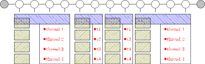
By the addition of extra communicators it has been possible to partition the work as follows. The
TNT_COMM_NETWORK group, shown in blue  , is the same distribution of the network as described in Section 4.
The hosts in this communicator hold the information about the network itself and follow the pTEBD algorithm. The
other hosts in the MPI job are split equally between these partitions. Each column, shown in green
, is the same distribution of the network as described in Section 4.
The hosts in this communicator hold the information about the network itself and follow the pTEBD algorithm. The
other hosts in the MPI job are split equally between these partitions. Each column, shown in green  , denotes a
TNT_COMM_SITE MPI communicator group of which there is a separate group for each partition of the network.
These processes have the lead processor being the one in TNT_COMM_NETWORK group. The other processors are held
waiting for a message from this ‘local’ root process to initiate a distributed SVD or matrix-matrix multiply
call.
, denotes a
TNT_COMM_SITE MPI communicator group of which there is a separate group for each partition of the network.
These processes have the lead processor being the one in TNT_COMM_NETWORK group. The other processors are held
waiting for a message from this ‘local’ root process to initiate a distributed SVD or matrix-matrix multiply
call.
It is worth noting that even though the root process may be running on a resource with as many cores as are included in the TNT_COMM_SITE group there is no reason why the full OpenMP threading of the non-LAPACK sections of the code cannot also use these cores since they would be idle at these times. These threads are denoted in Figure 4 in red.
In order to demonstrate the effectiveness of this approach in isolation from the other aspects of the software, Case 2 from Section 4 has been run with the blocking of the matrices for the SVD and the matrix-matrix multiply disabled. This gives a test case that enables us to test the performance of the SVD on a large range of matrix sizes.
The results for the cost of the SVD are shown in Figure 5
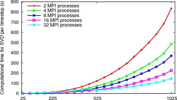
and the results for the matrix-matrix multiply routines look similar, with the maximum dual processor cost at 84s, i.e. about 10% of that of the SVD. It can be seen that a significant reduction in computational time is still being achieved up to 32 processes at the largest matrix size tested with over a minute extra being saved per timestep. The parallel efficiency of this approach appears to be a constant factor of 1.7 per doubling of the core count.
All the work developed in this project has been incorporated into the CCPForge repository [1], hence is available to users following the periodic releases of the updated code. Many of the features, such as the automatic blocking of the matrices and the reuse of the reshape calculations, are the defaults and are thus already being used to accelerate computations for all users.
In this project all three objectives have been met and all the target speed-ups have been obtained for serial execution. In addition use of OpenMP parallelism has been made outside the LAPACK call in order to optimise as much as the execution as possible. Distributed parallelism using MPI has also been applied in order to achieve concurrent computation of updates of different pairs of sites across the network. This has led to significant scalability being achieved in addition to the speed-ups from the other optimisations and techniques.
The changes made to the software have resulted in very minimal changes to user codes. Even the MPI routines are entirely hidden from the user enabling them to use these optimised features without knowledge of the communication taking place.
The parallel enhancements made in this software have also helped the developers to prepare for the next stages of their research. As was explained in the original proposal they are moving to working on 2-d networks. In fact they have now been funded for an EPSRC 5-year HPC Software Infrastructure grant to develop these capabilities building on the functionality added in this dCSE project. This work has successfully demonstrated that the software can run on HECToR with good utilisation of the machine.
This project was funded under the HECToR Distributed Computational Science and Engineering (CSE) Service operated by NAG Ltd. HECToR – A Research Councils UK High End Computing Service – is the UKs national supercomputing service, managed by EPSRC on behalf of the participating Research Councils. Its mission is to support capability science and engineering in UK academia. The HECToR supercomputers are managed by UoE HPCx Ltd and the CSE Support Service is provided by NAG Ltd. http://www.hector.ac.uk
[1] CCPForge website, http://ccpforge.cse.rl.ac.uk/gf/project/tntlibrary/
[2] S.R. White, Phys. Rev. Lett. 69, 2863 (1992).
[3] G. Vidal, Phys. Rev. Lett. 91, 147902 (2003); ibid 93, 040502 (2004).
[4] F. Verstraete, V. Murg, J.I. Cirac, Adv. Phys. 57, 143 (2008).
[5] I. Bloch, J. Dalibard, W. Zwerger, Rev. Mod. Phys. 80, 885 (2008).
[6] G. Vidal, Phys. Rev. Lett. 98, 070201 (2007).
[7] M. Suzuki, Phys. Lett. A 146, 6, (1990), ibid, J. Math. Phys. 32, 2, (1991).

![| |
|atmpRow [i],j|](finalreport11x.png)
![| |
|atmpRow [i],newCol[j]|](finalreport12x.png)