
HPC
Software for Massively Parallel Simulation of 3D Electromagnetic Nano-structures
A. Al-Jarro1,
C. G. Biris1,2, and N. C. Panoiu1
1Department of Electronic
and Electrical Engineering,
University College London, Torrington Place, London
WC1E 7JE, United Kingdom
2High Performance Computing Center, West University of Timisoara,
B-dul Vasile Parvan, Nr. 4, Timisoara
300223, Timis, Romania
Abstract
Advanced
research in photonic materials has shown that rapid breakthroughs in device
applications go hand-in-hand with the development of efficient, computationally
powerful software tools. Thus, high fabrication costs of complex photonic nano-structures and devices make it imperative to have
access to computational tools based on efficient algorithms, which can greatly
reduce the design-fabrication-testing cycle. In this context, computational techniques
based on the multiple-scattering formalism have become a primary means to model
a variety of scientific and engineering problems related to the electromagnetic
wave interaction with arbitrary distributions of particles and materials. In this work,
we have extended OPTIMET (OPTIcal
METa-materials) code, which is based on the 2D
multiple scattering matrix method, to allow for the analysis of electromagnetic
wave interaction with large ensembles of 3D micro- and nano-particles
that are periodically or arbitrarily distributed in an otherwise homogeneous
background. The newly developed software, OPTIMET-3D,
has the following additional functionalities, which dramatically enhance its
computational capabilities: (i) The extension of the
code capability to 3D photonic structures, (ii) The capability to model
non-linear (second-order) optical respons of
ensembles of particles, (iii) The capability to describe efficiently
periodically distributed electromagnetic scatterers,
(iv) The design and development of the software so as to render it suitable to
run efficiently on parallel HPC systems.
Table of Contents
4. The Multiple Scattering Matrix Method
4.1 Mathematical Formulation of the Multiple Scattering
Matrix Method
4.1.1 Single Particle Analysis
4.1.2 Multiple Particles System
4.1.3 Periodic Arrays of Particles
5. Technical Implementation of OPTIMET-3D
6. Performance and Scalability Analysis
7. Code Validation and Practical Examples
7.1 Single Particle Problem - Sphere
7.2 Validation of code implementation of the Vector
Translation-Addition Theorem
7.3 Two Particles Problem – Dimer
7.4 Super-Chirality from a Cluster of Dielectric
Nano-Spheres.
9. Conclusions and Future Work
1. Introduction
Over the past few years we have witnessed tremendous
progress in the design of photonic nano-materials, nano-devices and circuits, which in part has been greatly
accelerated by the availability of user-friendly, computationally powerful
software tools for device simulation and design. Advanced research in
integrated optics and photonics has shown that rapid, informed advances in
photonic device applications go hand-in-hand with the development of highly
efficient computational simulation tools. Thus, high fabrication costs of
complex photonic nano-devices make it imperative to
have access to computational tools based on efficient algorithms, which can
greatly accelerate the device design process and reduce the
design-fabrication-testing cycle. The future photonic
computational tools should be able to model a distributed multifunctional
device “continuum” in which the light is generated, processed and collected in
the same physical space. This complexity of the architecture of
photonics circuitry implies that future computational tools must fully
integrate the description of physical phenomena that take place over multiple
temporal, spectral and spatial scales. It is therefore evident that in order to
achieve rapid advances in nano-photonics, research in
computational methods and development of new and versatile HPC codes are of
crucial importance.
In recent years, computational
techniques based on the multiple-scattering formalism have become a primary
means for modelling a variety of scientific and engineering problems related to
the electromagnetic wave interaction with systems of particles and material
media [1-5]. Thus, computational methods based on the multiple-scattering
matrix (MSM) algorithm, also called the T-matrix
method, play a central role in modelling a vast array of applications, such as
photonic and plasmonic crystals (transmission, reflection,
absorption, density of states), metamaterials, nano-photonics (nano-lasers, plasmonic materials), radar signature technology, wireless
communications devices, antennae, microwave devices, bio-photonics and
biomedical imaging/treatment. The versatility of the MSM method allows one to
study the electromagnetic waves interaction with distributions of scatterers under a broad set of boundary conditions,
material parameters and geometries (periodic and non-periodic
boundary conditions, 2D and 3D geometries, in the time and frequency domains)
and can be applied to scattering systems that contain both linear and non-linear
media. More importantly, there is a scarcity of HPC
codes currently available on HECToR for
electromagnetic simulations (in fact, at the time of writing this report
we were aware of no such code). Similarly, on Legion (Legion@UCL, UCL's HPC compute
platform and the HPC system on which the code developed as
part of this project is intended to be used) there is only one HPC
electromagnetic simulator (MEEP), a time domain solver based on the FDTD
method.
2. Project Objectives
A versatile HPC tool for simulation of photonic materials must provide
two major capabilities: First, it should describe various geometries, which can
be 2D or 3D periodically or randomly arranged objects, a large variety of basic
building blocks of photonic materials and should provide a full
characterisation of the properties of the material both in the time and
frequency domains. Second, the HPC software should be efficient and easy to use
so as to appeal to a large user base. To this end, the main aim
of this project was to develop a versatile, easy to
use HPC software for massively parallel simulation both in the time and
frequency domains of 2D and 3D materials that are periodically or randomly
structured. The proposed
software development work has been organised along three major work packages:
Work
package 1: Extension of OPTIMET to 3D structures
This part of the project was
devoted to the extension of the current OPTIMET code [5] to 3D geometry.
·
Incorporate in the code vector spherical wave functions (VSWF) via the addition of spherical harmonic functions;
·
Implement the functions that construct the scattering matrix of
the system and the 3D fields. The scattering matrix of the system is
constructed at node level whilst the spectral and time domain calculations are
implemented via MPI and distributed across the
available nodes.
·
Implement the functions that compute the system
cross-sections. This task amounted to writing the routines for calculating the
total, scattering and absorption cross-sections of the system.
Work package 2: Implementation of
periodic boundary conditions
In this part of the project the
periodic boundary conditions capability was added to the code.
·
Implement the routines to compute the transmission/reflection
matrices.
·
Implement the functions for the transmission/reflection matrices
of a set of layers of scatterers.
·
Implement the routines that compute the transmission and
reflection coefficients of a material slab.
Work
package 3: Extension of OPTIMET so as to incorporate quadratic nonlinearities
OPTIMET-3D was developed to
incorporate the effects induced by quadratic optical nonlinearities.
·
Write a set of routines for computing the nonlinear scattering
matrix of the system.
·
Write the functions that compute the total, scattering
and absorption cross-sections of the system.
We want to mention here that originally we intended to
implement the simpler case, namely, that of cubic (Kerr) optical
nonlinearity. However, as the project progressed, it became clear
that we would be able to develop a branch of the code for modelling the much
more complex case (and more important from a practical point of view), that of quadratically non-linear optical interactions. The main reason for this
change in strategy was that the developer of the original version of the code,
Dr Claudiu Biris, was able
to invest in this project more time than it has been originally anticipated.
3. Project Outcomes
The main outcomes of the project can be divided in
two main categories, namely, a versatile HPC software (OPTIMET-3D) that can
accurately model the interaction between electromagnetic waves and arbitrary
distributions of metallic, dielectric and semiconductor particles, and an
enhanced capability to investigate and solve a multitude of scientific problems
that are relevant to several areas of science and technology, including
optoelectronics, photonics, materials science, plasmonics,
nanotechnology, non-linear optics and surface science. In fact, we have already
used OPTIMET-3D to demonstrate for the first time that, surprisingly,
super-chiral light can be generated in clusters of silicon nano-spheres;
a conference paper on this topic will be presented shortly after the completion
of the project [6].
OPTIMET-3D has been
developed to be used on Legion (Legion@UCL) UCL's HPC
cluster. Legion comprises 904 nodes offering over
5600 processor cores, each with between 2GB and 4GB RAM. Most of the system is
connected by high-performance interconnect. The cluster is coupled to a
large-scale high-performance file system, with a total capacity of 192 TB. The
cluster features a range of best-in-class compilers and related tools for
serial and parallel code development, such as Intel C++ and FORTRAN compilers, Pathscale Compiler Suite, a broad set of libraries, such as
Intel's Math Kernel Library (MKL), BLACS, LAPACK and ScaLAPACK,
and software tools for development of parallel code, such as MPICH2 and OpenMP. The service is currently further expanded, with new
compute capacity being added to the cluster. The current version of OPTIMET-3D
deployed on Legion was built using Intel’s Compiler
Collection version 11.1 and uses the OpenMPI 1.4.1
parallel library suite.
OPTIMET-3D has also been
successfully ported and run on two other HPC platforms, specifically, the InfraGrid and BlueGene/P clusters
at the West University of Timisoara (Romania). InfraGrid
is an Intel® Xeon cluster with 100 Quad Core CPUs clocked at 2.0 GHz. Each CPU
has direct access to 10 GB of RAM and all share a 145 GB SAS local storage
device. The system uses 40Gbps 4xQDR Infinipath
interconnect to ensure fast and stable inter-node communications. OPTIMET-3D
was deployed on InfraGrid using Intel’s Compiler
Collection version 11.1 and uses Intel’s MPI 4.1 library. The second HPC
platform is a BlueGene/P rack with 1024 Quad Core
PowerPC-450 processors. Each CPU has access to 4GB of RAM and the cluster is
connected to a 48×320 GB SAS IBM DS3524 networked storage arrays. Interconnect
is provided by a Torus 3D network. To date, OPTIMET-3D has been tested on the BlueGene/P cluster but no production code has been run.
These tests have been performed to ensure compatibility with IBM technologies,
specifically, MKL was replaced by IBM’s Engineering and Scientific Subroutine Library
(ESSL) and the code was compiled with IBM’s XL Compiler Suite, version 9.0, and
linked with the IBM MPIx parallel library.
After full testing,
OPTIMET-3D will be hosted at http://www.ee.ucl.ac.uk/~npanoiu/Software.html,
on Dr Panoiu's webpage at UCL, and will be freely
available for download. The software will also be made freely available to all
interested users of Legion. In
order to increase the dissemination and potential use of the software, we are
also preparing a journal article that will be submitted together with the code
to Comp. Phys. Comm. journal. OPTIMET-3D is
currently stored on BitBucket in a Mercurial repository (https://bitbucket.org/cbiris/optimet3d).
Access to it is available through any compatible Mercurial client that can
access Mercurial repositories of version 1.4 or higher, such as “hg” for Unix or Tortoise HG for Windows. The current version of OPTIMET-3D
has about 20500 lines of code. We use the following four branches, for
development and code release:
·
default – this is the default branch, which contains the
current release version of OPTIMET-3D and also incorporates the previous
software, OPTIMET. This branch would be accessed by users who are interested in
using OPTIMET-3D, but do not wish to develop code using the API.
·
devel – this is the main development branch for the serial
version of the code. This version contains all the latest features of the code,
as they are first tested in the serial version before being pushed onto the
parallel development branch.
·
devel-parallel – this is the main development branch
for the parallel version of the code. This branch is a mirror of the devel branch but contains
parallel version of the needed functions and classes. Since features are tested
in the serial version first, this branch may occasionally have less features than the devel branch.
·
forward – this is a private branch which is used only by the
OPTIMET-3D developers to implement and perform initial tests of new features in
future release versions of the code. Understandably, some of the features in
this branch may be unstable or untested, so users who want to use OPTIMET-3D
API should synchronise with the devel
or devel-parallel branches
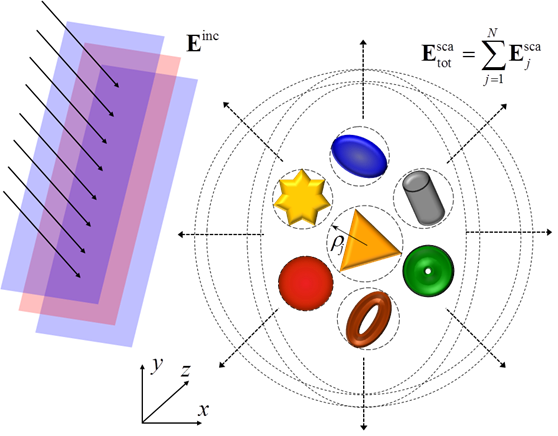
Figure
1. Schematic representation of the incident
field/scattered field theoretical model and 3D structure of a cluster of
arbitrary scatterers.
The software tool
developed as part of this project has three major capabilities, which have been
implemented as part of the three major thrusts (work packages) of the software
development work. The corresponding blocks of the code that implement these main
features are parallelised. All parts of the source code are integrated in a
single software tool, which makes it particularly easy to use and disseminate
the code and to further develop it as well.
First, unlike the previous version (OPTIMET), the HPC
code can now model fully 3D electromagnetic structures (as schematically shown
in Fig. 1). This represents a dramatic improvement of the code, particularly
from a practical point of view. The electromagnetic scatterers
can have rather arbitrary shape, including spheres, ellipsoids and pyramids.
Additional shapes can be modelled by simply providing the parametric
representation of the corresponding surface of the scatterer.
Moreover, the scatterers can have different size, can
be arbitrarily distributed and can consist of materials with different
electromagnetic properties, provided via the
electrical permittivity (e) and magnetic permeability (m).
Once the configuration of the incoming field (direction and polarisation) and
distribution of scatterers are provided, OPTIMET-3D
can compute the main physical quantities of interest, namely, electromagnetic
field distribution and the scattering cross-section, absorption cross-section
and the total (extinction) cross-section. Importantly, since the frequency enters
into the computations only through the electromagnetic constants of the
particles (scatteres) OPTIMET-3D can practically be
used for any frequency in the electromagnetic spectrum.
The second major feature
of OPTIMET-3D is that it can describe the interaction of electromagnetic waves
with periodic distribution of particles. This feature makes it particularly
useful in studies of optical properties of photonic and plasmonic
crystals and, more generally, for modelling photonic meta-materials. In
particular, the software tool can be used to compute the transmission and
reflection coefficients of a slab of photonic material and, consequently, the
optical absorption in the slab, as well as the photonic band structure of the
photonic material. As in the previous case, the particles in the unit cell can
have arbitrary shape and size and can be made of various optical materials,
including metals, semiconductors and dielectrics.
The third major
capability of OPTIMET-3D is that it can describe the non-linear interaction
between electromagnetic waves and arbitrary distributions of particles made of centro-symmetric optical materials, such as noble metals
and silicon. In this non-linear optical interaction, the
electromagnetic field at the fundamental frequency (w)
gives rise to a field at the second harmonic (2w),
the field generation being confined primarily at the surface of particles or
interfaces. This is perhaps the most important optical effect in
non-linear optics, with many applications in surface optical spectroscopy,
surface chemistry and optical biosensing. As in the
linear case, the code provides the main physical quantities that characterise
the (non-linear) interaction between the electromagnetic field and arbitrary
distributions of particles, that is, the electromagnetic field distribution and
the scattering cross-section, absorption cross-section and the extinction
cross-section. We mention here that originally we intended to implement the
simpler case, namely, that of cubic optical nonlinearity.
In addition to a
high-performance, versatile code, this project has another major outcome,
namely, it would play an important role in enhancing current scientific
collaborations with worldwide leading academic groups working in nano-photonics and help to start new ones as well. In fact,
we have already identified potential collaborations with Prof Jeremy Baumberg and Dr Ventsislav Valev from the University of Cambridge, in which OPTIMET-3D
will be used to interpret experimental data regarding optical properties of
self-assembled clusters of metallic nano-particles
(more details about the scientific use of OPTIMET-3D are given in Sec. 7).
·
As part of our ongoing
research collaboration with Dr Paul Warburton’s Group at UCL and Prof Richard
Osgood’s Group at Columbia University we plan to use OPTIMET-3D to study the
non-linear optical properties of plasmonic
meta-materials and non-linear photonic crystals. In particular, the software
tool will be instrumental in advancing our work on next-generation solar cells
that incorporate plasmonic materials.
·
We will use OPTIMET-3D in our ongoing
collaboration with Prof Chee Wei Wong's group at
Columbia University, on multi-colour Anderson wave localisation in disordered
ensembles of dielectric nano-particles.
·
QPTIMET-3D will be instrumental in our ongoing collaboration with Prof Shuang
Zhang's group at the University of Birmingham and Prof Xiang Zhang's group at
Berkeley University (USA), a project supported by
EPSRC/NSF (EP/J018473/1),
on optical properties of classical and quantum meta-materials.
4. The Multiple Scattering Matrix Method
In
order to facilitate the understanding of the main capabilities of OPTIMET-3D,
we briefly present in this section the numerical method on which the code is
based. Thus, the main steps of the MSM method can be described as follows:
First, the incident, scattered, and internal (inside the scatterers)
fields are expanded in Fourier series. The basis
functions in 2D and 3D are multipole functions and
VSWF, respectively [2-5]. Then, one constructs a system of linear equations
whose unknowns are the Fourier coefficients of the scattered field. These
coefficients are the main unknowns of the scattering problem as they can be
used to compute most of the main physical quantities characterising the wave
interaction, namely, the electromagnetic field distribution both inside and outside the scatterers, and the scattering, absorption and the
extinction cross-sections.
This
brief description of the MSM method shows that the main part of this algorithm
consists in constructing and solving a system of linear equations whose
unknowns are the Fourier coefficients of the scattered field. The matrix
defining this system, also called the transfer matrix
(or T-matrix), is completely defined by the
location, shape and material parameters of the particles. The T-matrix of the system has a block structure, the
corresponding blocks consisting of single-particle T-matrices
and matrices that describe inter-particle interactions (coupling between
particles). As a consequence of this block structure of the T-matrix, the MSM method can be easily applied to clusters
with different number and distribution of particles. Equally important, the obvious scalability with the
number of particles renders the MSM algorithm particularly suitable for
parallelisation.
4.1 Mathematical Formulation of the Multiple
Scattering Matrix Method
Consider
a cluster of N particles being illuminated by
a monochromatic plane electromagnetic wave. The origin of the co-ordinate
system of the cluster is ![]() and to each particle (j)
one associates a co-ordinate system with the origin,
and to each particle (j)
one associates a co-ordinate system with the origin, ![]() . The only constraint imposed on the
location of the particles is that the circumscribing spheres of the particles
do not overlap, i.e.
. The only constraint imposed on the
location of the particles is that the circumscribing spheres of the particles
do not overlap, i.e. ![]() ,
, ![]() , where as per Fig. 1
, where as per Fig. 1 ![]() is
the radius of the smallest sphere containing the jth particle.
is
the radius of the smallest sphere containing the jth particle.
The solution of the
source-free Maxwell equations in 3D can be expanded in a complete basis of
VSWFs, ![]() and
and ![]() . In a practical implementation, the
series is truncated to a certain order,
. In a practical implementation, the
series is truncated to a certain order, ![]() . Let
. Let ![]() then, the incident, scattered and internal
electric fields can be expressed as [2-5]:
then, the incident, scattered and internal
electric fields can be expressed as [2-5]:
incident field

internal field

scattered field

where ![]() and
and ![]() are the wave vectors in the embedding medium
and inside the jth
particle, respectively,
are the wave vectors in the embedding medium
and inside the jth
particle, respectively, ![]() and
and ![]() ,
,![]() , are the position vectors of a point, P, in the co-ordinate systems
, are the position vectors of a point, P, in the co-ordinate systems ![]() and
and ![]() , respectively. The magnetic field is
subsequently obtained from the electric field as
, respectively. The magnetic field is
subsequently obtained from the electric field as ![]() . The unknown expansion coefficients of
the internal and scattered fields,
. The unknown expansion coefficients of
the internal and scattered fields, ![]() and
and ![]() , respectively, can be expressed in terms
of the known expansion coefficients of the
incident monochromatic plane wave,
, respectively, can be expressed in terms
of the known expansion coefficients of the
incident monochromatic plane wave, ![]() , by imposing at the surface of the
particles the boundary conditions satisfied by the electric and magnetic
fields.
, by imposing at the surface of the
particles the boundary conditions satisfied by the electric and magnetic
fields.
In the non-linear case, the corresponding electric
field at the fundamental frequency (FF), ![]() , gives rise to an electromagnetic field
at the second harmonic (SH) frequency,
, gives rise to an electromagnetic field
at the second harmonic (SH) frequency, ![]() . This field is generated by the
non-linear dipoles described by the non-linear polarisation,
. This field is generated by the
non-linear dipoles described by the non-linear polarisation, ![]() [5,7,8]:
[5,7,8]:
![]()
surface polarization
![]()
bulk polarization
![]()
For
a rigorous derivation of Eqs. (5) the reader
is referred to [8].
4.1.1 Single Particle Analysis
Let ![]() , with
, with ![]() , be a column vector, and define
similarly
, be a column vector, and define
similarly ![]() ,
, ![]() ,
, ![]() ,
, ![]() and
and ![]() . Here,
. Here, ![]() ,
, ![]() and
and ![]() represent the Fourier expansion coefficients
of the incident, internal and scattered fields, respectively,
defined with respect to
represent the Fourier expansion coefficients
of the incident, internal and scattered fields, respectively,
defined with respect to ![]() , relative to
, relative to ![]() ,
, ![]() . Moreover, if one assumes that the
system contains only the
. Moreover, if one assumes that the
system contains only the ![]() th particle, a compact matrix
representation of the Fourier coefficients of the electromagnetic fields, both
inside and outside the particle, can be cast as follows [2]:
th particle, a compact matrix
representation of the Fourier coefficients of the electromagnetic fields, both
inside and outside the particle, can be cast as follows [2]:
 (6)
(6)
Here, ![]() and
and ![]() ,
, ![]() , are the scatterer-centred T-matrix of the jth
particle and a matrix that relates the Fourier coefficients of the inside and
outside fields, respectively. Note that the block-diagonal structure of the
, are the scatterer-centred T-matrix of the jth
particle and a matrix that relates the Fourier coefficients of the inside and
outside fields, respectively. Note that the block-diagonal structure of the ![]() and
and ![]() matrices is valid only for spherical
particles.
matrices is valid only for spherical
particles.
4.1.2 Multiple Particles System
The central idea of the Foldy–Lax multiple scattering theory [9] is that in the
vicinity of any scatterer ![]() in the
in the ![]() particle system, there is a local field that
is the superposition of the incident field and the field scattered by all the
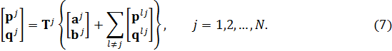
other scatterers in the system, except the scatterer itself. Using the definition of the
single-particle T-matrix,
particle system, there is a local field that
is the superposition of the incident field and the field scattered by all the
other scatterers in the system, except the scatterer itself. Using the definition of the
single-particle T-matrix, ![]() ,
, ![]() , the Fourier expansion coefficients of the
scattered and incident fields,
, the Fourier expansion coefficients of the
scattered and incident fields, ![]() and
and ![]() , respectively, obey the following
equation:
, respectively, obey the following
equation:
The coefficients ![]() and
and ![]() , where
, where ![]() , and similarly for
, and similarly for ![]() , need to be expressed in terms of the
known expansion coefficients of the incoming field and
, need to be expressed in terms of the
known expansion coefficients of the incoming field and ![]() , respectively, which are calculated in
the system with the origin in
, respectively, which are calculated in
the system with the origin in ![]() . This is achieved by using the vector
translation-addition theorem [2, 4]. Thus, let us consider the matrix
coefficients,
. This is achieved by using the vector
translation-addition theorem [2, 4]. Thus, let us consider the matrix
coefficients,
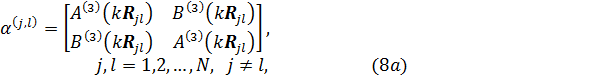
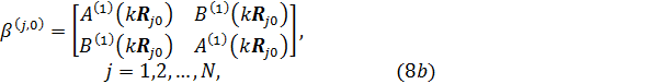
where ![]() and
and ![]() ,
, ![]() , represent the vector
translation-addition coefficients, which are evaluated using an efficient
recursive implementation as proposed in [4]. Let
, represent the vector
translation-addition coefficients, which are evaluated using an efficient
recursive implementation as proposed in [4]. Let ![]() and
and ![]() . Then, the single-particle scattering
expansion coefficients,
. Then, the single-particle scattering
expansion coefficients, ![]() , can now be expressed
in terms of
, can now be expressed
in terms of ![]() and
and ![]() ,
, ![]() , as:
, as:

In terms of the known
Fourier expansion coefficients of the incident field, ![]() , the resulting system of linear
equations for the
, the resulting system of linear
equations for the ![]() particle system for the unknown Fourier
expansion coefficients of the scattered field,
particle system for the unknown Fourier
expansion coefficients of the scattered field, ![]() ,
, ![]() , can be expressed in the following form:
, can be expressed in the following form:
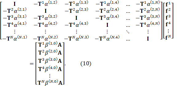
The system (10) can be
expressed in a compact matrix form, ![]() , where
, where ![]() ,
, ![]() and
and ![]() denotes the FF (linear) scattering
matrix of the system. Constructing the system
matrix
denotes the FF (linear) scattering
matrix of the system. Constructing the system
matrix ![]() and solving Eq. (10)
represent the core parts of the MSM method. Similarly, in the non-linear case the
scattering problem is reduced to solving a system of linear equations,
and solving Eq. (10)
represent the core parts of the MSM method. Similarly, in the non-linear case the
scattering problem is reduced to solving a system of linear equations, ![]() , where
, where ![]() and
and ![]() are the (non-linear) scattering matrix of the
system and the Fourier
expansion coefficients of the (non-linear) scattered field, respectively.
are the (non-linear) scattering matrix of the
system and the Fourier
expansion coefficients of the (non-linear) scattered field, respectively.
4.1.3 Periodic Arrays of Particles
Consider an infinitely
extended, 2D periodic lattice of particles situated in the xy-plane, defined by the Bravais
lattice vectors ![]() , where
, where ![]() and
and ![]() are the basis vectors of the lattice. The
corresponding reciprocal lattice is defined by
are the basis vectors of the lattice. The
corresponding reciprocal lattice is defined by ![]() , where
, where ![]() and
and ![]() are the basis vectors of the reciprocal
lattice.
are the basis vectors of the reciprocal
lattice. ![]() and
and ![]() are related through the relations
are related through the relations ![]() .
.
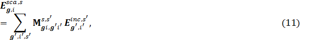
The solution for the
scattered electromagnetic field for an arbitrary 2D lattice can be efficiently
obtained via the lattice-centre
translation-addition theorem, which replaces the contribution of each particle
with an equivalent contribution of a particle located at ![]() [10,11]. Then, the total scattered field,
[10,11]. Then, the total scattered field, ![]() , is obtained from the reciprocal lattice
identity relationship, which expresses the VSWFs expansion in the
, is obtained from the reciprocal lattice
identity relationship, which expresses the VSWFs expansion in the ![]() lattice
in the limit
lattice
in the limit ![]() in
an equivalent form as a truncated expansion in the reciprocal lattice [10,11]:
in
an equivalent form as a truncated expansion in the reciprocal lattice [10,11]:
scattered field
where ![]() and
and ![]() denote Cartesian components,
denote Cartesian components, ![]() denote the direction of the incident field,
denote the direction of the incident field, ![]() , for
, for ![]() and
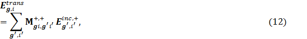
and ![]() . The analytical expressions for
. The analytical expressions for ![]() are given in [10,11].
From these expressions the transmitted and reflected
fields from the 2D lattice are:
are given in [10,11].
From these expressions the transmitted and reflected
fields from the 2D lattice are:
transmitted field
reflected field
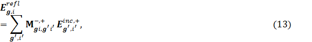
where the corresponding transmittance and
reflectivity of the 2D lattice (slab) are defined as the ratio of the fluxes of
![]() and
and ![]() , respectively, to the flux of
, respectively, to the flux of ![]() (note that the sum over the diffraction orders
(note that the sum over the diffraction orders
![]() has been taken out). The details of the
implemented code, OPTIMET-3D, and the associated parallelisation strategy are
presented in the next section.
has been taken out). The details of the
implemented code, OPTIMET-3D, and the associated parallelisation strategy are
presented in the next section.
5. Technical Implementation of OPTIMET-3D
In this
section, the technical implementation of OPTIMET-3D and several parallelisation
strategies employed for its numerical acceleration are presented. Then, the
structural framework of the software is given with a comprehensive description
of the major building blocks of the code.
5.1 Technical Overview
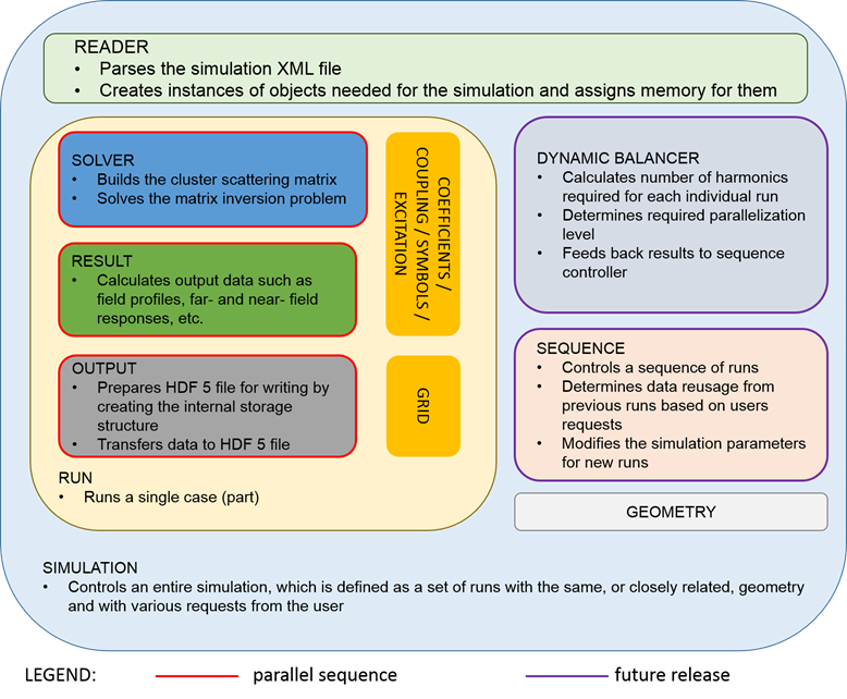
Figure
2. Structural block-diagram of OPTIMET-3D. Each block in the
framework of the code corresponds to a single C++ class.
In the code development work, we used DOXYGEN
documentation system, which integrates very well within the OOP framework. It
dynamically generates an interactive documentation of the resulting API. The
associated documentation is available in both HTML and PDF formats.
For the end users, those who do not intend to develop
their own simulations using the API, OPTIMET-3D has a very simple and flexible
input system based on a single XML file. For this, we use pugixml,
a lightweight and fast, open source XML parser that can be found at https://code.google.com/p/pugixml/.
The user is required to define XML blocks such as simulation parameters,
geometry and incoming wave. Each of these blocks contains sub-blocks, which can
hold, for example, object definitions such as position, electromagnetic
properties, particle size, etc. A short guide explaining how to write an input
file is made available with the code. It should be noted that due to the
popularity of XML as a data description solution, many graphical interfaces
exist for building XML files. Therefore, it would be trivial to create a
user-friendly GUI for all data input.
In terms of deployment,
we use the CMake
system in order to enhance the portability of OPTIMET-3D and facilitate its
installation on a given HPC system. CMake is an
automated makefile
generator, which searches for existing libraries on the target system and
builds an appropriate makefile
to compile the software. Currently, OPTIMET-3D requires four major components
for it to work: an MPI library, a mathematical library that offers LAPACK and
BLAS (ScaLAPACK, PBLAS and BLACS for the parallel
version), the GNU Scientific Library and the HDF5 library. CMake
uses finders, which are simple script files,
to locate static and dynamic objects, as well as header files. Currently, the finders support OpenMPI, Intel's
MPI and MPICH for the parallel communication libraries, and Intel’s MKL, IBM’s
ESSL and the Armadillo Linear Algebra Pack for accessing the mathematical
subroutines. Finally, it should be noted that both GSL and HDF5 are open-source
packages, which are available on most scientific computing systems.
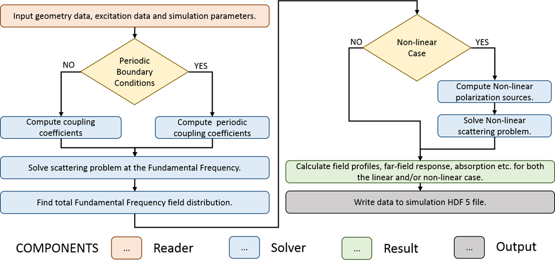
Figure 3. Workflow of an
OPTIMET-3D simulation.
In order not to burden the user with editing makefiles
or to be concerned over the resulting linkage order and linking targets, the CMake system provides ideal functionality for improved code
portability. The associated CMake scripts have been
tested on several HPC platforms, so far, including UCL’s Legion
and the InfraGrid and BlueGene/P
HPC systems at the West University of Timisoara. Moreover, it is rather
straightforward to manually add additional support for a new system or library.
For example, in order to add support for the AMD’s mathematical libraries, the
user simply has to change the linear algebra finder script in order to point to
these new libraries. In addition, in the use of CMake,
the user has the option to specify a number of flags in order to indicate support for
the statically or dynamically linked libraries and to choose the parallel or
serial branch of the code.
Finally, we use the Mercurial revision control system
in order to facilitate access to all revisions of the code, as well as the up
to date API documentation.
5.2 Structural Framework
As we have explained,
OPTIMET-3D strictly follows OOP framework guidelines. Specifically, each single
component of the code is defined as a separate class with its own header file.
Classes that have to perform data storage operations are given two main access
methods, an init() method, which allocates any necessary memory for the
data storage and initialises the object, and a populate() method, which populates the data storage
attributes of the object based on the initialisation parameters and the role of
the object. Classes that have no data storage role are declared with all
members static in order to allow easy access to them and eliminate
any confusion as to the need of instantiation. A schematic overview of the
structural framework of OPTIMET-3D is presented in Fig. 2, whereas the workflow
associated with a typical OPTIMET-3D simulation and the corresponding features
of the code are shown in Fig. 3.
The main classes defined
in the framework of OPTIMET-3D are:
·
Algebra – defines wrappers to linear algebra and vector-vector and
vector-matrix operations solvers based on the available mathematical libraries
(currently supports BLAS, LAPACK, GSL, MKL, ESSL, Armadillo); includes parallel version.
·
Coefficients – computes all expansion coefficients needed for vector spherical
components, including the ![]() and
and ![]() vector functions, and the Wigner d-functions.
vector functions, and the Wigner d-functions.
·
Coupling – computes electromagnetic coupling coefficients between particles,
specifically, ![]() and
and ![]() transfer matrix coefficients, which are
used to transform vector spherical functions between co-ordinate systems.
transfer matrix coefficients, which are
used to transform vector spherical functions between co-ordinate systems.
·
PeriodicCoupling – this class is identical to the Coupling class in terms of usage and scope, but it
is used as a replacement for the former when periodic boundary conditions are
employed in simulations.
·
Excitation – defines an incoming electromagnetic excitation, including
expansion coefficients and polarisation state (currently supports plane wave
excitations with Gaussian pulsed excitation [12] being planned for a future
release).
·
Geometry – stores all data defining the cluster geometry (including
electromagnetic properties). It also stores for each scatterer
the Fourier expansion coefficients of the internal electromagnetic fields.
·
Output – provides a versatile interface to set up the internal structure
of the HDF5 output file of the simulation, as well as input/output data
transfer to this file; includes parallel version.
·
OutputGrid – defines spatial grids for 3D field output
and visualisation. The current version supports regular and iregular
cartesian grids. Spherical and cylindrical co-ordinate grids will be provided
in a future release.
·
Reader – parses the simulation XML file and sets up all of the needed
objects, including the Geometry, Excitation, Output and OutputGrid objects (the latter one is used only in
cases where field results are requested).
·
Result – calculates required physical data from the Fourier expansion
coefficients (i.e. scattering and internal
expansion coefficients) provided by the Solver. Currently the software calculates field
profiles, near- and far-field cross-sections, and performs wavelength scans; includes parallel version.
·
Run – provides an interface to run a single instance of the solver (i.e. using a fixed geometry and excitation source).
·
Simulation – overall control and monitoring class. Ideally, this should be
the only class with which a user of the API needs to interact directly, as once
instantiated it provides access to the Geometry, Excitation, Solver, Result and Output classes.
·
Solver – solves system of linear equations corresponding to the linear or
non-linear scattering problem and feeds the solution to a Result object; includes
parallel version.
·
Symbol - provides static members to compute several symbols and special
functions required by the numerical formalism (e.g.,
3j, 6j and 9j Wigner symbols, Clebsch-Gordan
coefficients and the ![]() -symbols required for computing the non-linear sources).
-symbols required for computing the non-linear sources).
·
Sequence – provides an interface that allows the user to create a series of
requests from the simulation point of
view (e.g., specific field profiles,
cross-sections, wavelength scans, etc.). The role of this class is to ensure
that no extra work is being spent on computing any data that may not be needed
(e.g., there is no point in calculating
the internal field coefficients when only the linear far-field response is
requested).
·
Balancer – provides a dynamic balancer that, for each scatterer,
automatically calculates the maximum number of harmonics required for
convergence (based on the electromagnetic and geometrical properties of the
particular scatterer). This in turn determines the
level of parallelisation required, based on the number of scatterers
and nodes available, as well as the resources allocated to each node. The
outcome is then fed back to the Sequence controller; this class is planned for
a future release as it requires comprehensive testing.
5.3 Parallel Implementation
The basic characteristics of the multiple scattering matrix method renders
the algorithm implemented as OPTIMET-3D highly parallelisable, scalable and
stable. The software setup does not suffer from race conditions and
encapsulates highly uniform data structures, which potentially allow for
straightforward achievement of load balancing.
The primary challenge that arises when performing
complex numerical simulations, namely, those which involve the study of a large
number of scatterers, is the need for a large amount
of memory required for storing the system scattering matrix, i.e. ![]() or
or
![]() . In order to illustrate these memory
requirements, the size of the scattering matrix approaches 6 GB for a cluster
of 13 particles with
. In order to illustrate these memory
requirements, the size of the scattering matrix approaches 6 GB for a cluster
of 13 particles with ![]() harmonics. In our calibration, this is
considered a large memory requirement, in particular, when considering a
parallel clusters where, typically, the per node memory
size ranges between 2 GB and 4 GB. In addition, as the distance between any two
scatterers in the cluster increases, in order to
obtain accurate convergence in the VSWF translation calculations,
harmonics. In our calibration, this is
considered a large memory requirement, in particular, when considering a
parallel clusters where, typically, the per node memory
size ranges between 2 GB and 4 GB. In addition, as the distance between any two
scatterers in the cluster increases, in order to
obtain accurate convergence in the VSWF translation calculations, ![]() must be increased as well. To be more specific, in some cases up to 40
harmonics or more may be required. Furthermore, as several of our envisioned
science related applications of OPTIMET-3D will require randomly distributed
ensembles of hundreds of particles, employing a distributed computing method
relying on splitting the memory cost of storing the scattering matrix among
available nodes becomes mandatory.
must be increased as well. To be more specific, in some cases up to 40
harmonics or more may be required. Furthermore, as several of our envisioned
science related applications of OPTIMET-3D will require randomly distributed
ensembles of hundreds of particles, employing a distributed computing method
relying on splitting the memory cost of storing the scattering matrix among
available nodes becomes mandatory.
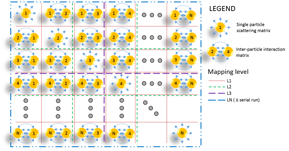
Figure 4. Diagram of the parallelisation
scheme for the cluster scattering matrix for N scatterers.
Depending on the mapping level, each node stores and processes from 1 to N
blocks of the global matrix.
The algorithm used to
distribute the memory is schematically depicted in Fig. 4. The most basic and
most natural memory split is per bi-particle
interaction level. Each node holds the part of the matrix that
describes either the single scattering matrix, ![]() , or the inter-particle interaction
matrix. We denote this scheme as Level 1
(L1) parallelisation strategy. While L1 is straightforward to implement and
uses efficiently the intrinsic symmetries in the scattering matrix formalism,
it has several drawbacks. First, whilst the cluster scattering matrix is large,
the distributed components only take a few hundreds of MB in memory storage,
thus, each node only uses a fraction of its available resources. Second, the
number of required nodes scales quadratically with
the number of scatterers in the system. As a result,
for the relatively simple case of a cluster with 20 particles, 400 nodes are
required to implement an L1 parallelisation strategy. For HPC systems of the
size of Legion this might not be practical (on Legion the cores requirement of a typical job cannot exceed
~200).
, or the inter-particle interaction
matrix. We denote this scheme as Level 1
(L1) parallelisation strategy. While L1 is straightforward to implement and
uses efficiently the intrinsic symmetries in the scattering matrix formalism,
it has several drawbacks. First, whilst the cluster scattering matrix is large,
the distributed components only take a few hundreds of MB in memory storage,
thus, each node only uses a fraction of its available resources. Second, the
number of required nodes scales quadratically with
the number of scatterers in the system. As a result,
for the relatively simple case of a cluster with 20 particles, 400 nodes are
required to implement an L1 parallelisation strategy. For HPC systems of the
size of Legion this might not be practical (on Legion the cores requirement of a typical job cannot exceed
~200).
In addition to the L1 parallelisation
scheme, where each basic block is distributed to a node, higher levels of
matrix distribution have been considered, as illustrated in Fig. 4. Each level
Lm distributes an
![]() block matrix to each node. In
this notation, for a given cluster with
block matrix to each node. In
this notation, for a given cluster with ![]() particles, when
particles, when ![]() the algorithm implementation simply becomes a
serial one. Thus, by allowing a flexible use of higher-order
parallelisation levels, OPTIMET-3D software can use efficiently the available
resources whilst allowing complex simulations to run
on smaller number of nodes. We refer to this type of parallel mapping as balanced mapping.
the algorithm implementation simply becomes a
serial one. Thus, by allowing a flexible use of higher-order
parallelisation levels, OPTIMET-3D software can use efficiently the available
resources whilst allowing complex simulations to run
on smaller number of nodes. We refer to this type of parallel mapping as balanced mapping.
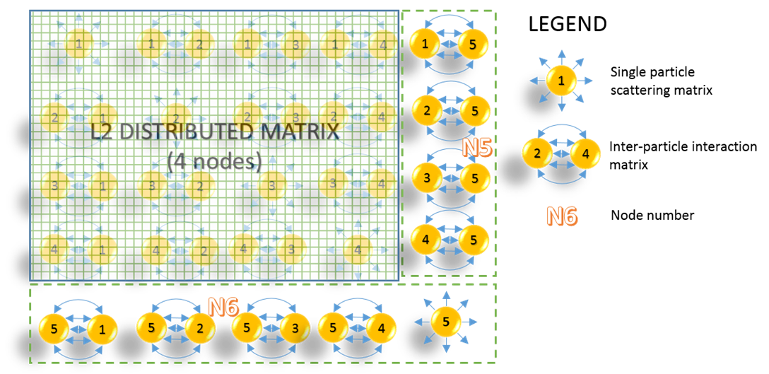
Figure 5. Example of “edge” distribution
of the scattering matrix elements in an unbalanced mapping case. The
geometry consists of 5 particles. The first 4 blocks of the scattering matrix
are mapped with the L2 scheme whilst the remaining blocks are distributed as
shown.
One issue that arises
with a higher level of parallelisation is the unbalanced distribution of the
scattering matrix when it is not exactly mapped to the available nodes by
square-block matrices (i.e. when the
number of scatterers N
is not an integer multiple of the parallelisation level m).
This situation is illustrated in Fig. 5. To simplify the presentation of this
case, consider a very basic cluster of 5 scatterers,
whose scattering matrix contains ![]() elemental blocks. The first 16 elemental
blocks of the 25 block matrix are distributed according to an L2 mapping,
whereas the remaining 9 blocks are mapped as a column and row block matrices.
Note that the last node will have an additional block to process. This is
usually of a limited concern since the corresponding block components are
independent. Therefore, no race condition occurs. It has been observed during
our numerical experiments that for
elemental blocks. The first 16 elemental
blocks of the 25 block matrix are distributed according to an L2 mapping,
whereas the remaining 9 blocks are mapped as a column and row block matrices.
Note that the last node will have an additional block to process. This is
usually of a limited concern since the corresponding block components are
independent. Therefore, no race condition occurs. It has been observed during
our numerical experiments that for ![]() , a
, a ![]() matrix requires less than 2 GB, thus making
very useful the L4 and L3 mapping schemes. As a consequence, this edge mapping scheme can be used for particle clusters that
have the property
matrix requires less than 2 GB, thus making
very useful the L4 and L3 mapping schemes. As a consequence, this edge mapping scheme can be used for particle clusters that
have the property ![]() , where
, where ![]() is
an arbitrary integer. In addition, edge mapping can be used for any odd number
of scatterers. Nevertheless, for
is
an arbitrary integer. In addition, edge mapping can be used for any odd number
of scatterers. Nevertheless, for ![]() , the resulting size of a block is less
than 1 GB. This makes the Lm scheme
practical for the relatively older generation of computing systems; however, it
may lead to resource wasting on newer clusters. To this end, the following hybrid mapping scheme is proposed.
, the resulting size of a block is less
than 1 GB. This makes the Lm scheme
practical for the relatively older generation of computing systems; however, it
may lead to resource wasting on newer clusters. To this end, the following hybrid mapping scheme is proposed.
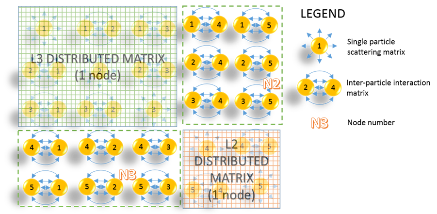
Figure 6. Schematic of the hybrid mapping
strategy. The example considered is for N=5 particles. Note that this is
one of several possible hybrid mapping strategies for this particular N.
The hybrid mapping scheme
combines several balanced mapped areas of different levels, as well as row and
column mapping in order to cover the entire scattering matrix of the system, as
per Fig. 6. The hybrid mapping scheme proves to be the most effective mapping
model in terms of resource balancing. However, one does not expect the user to
create the corresponding map, so that an automatic mapping scheme must be
implemented. As a result, this is no longer as simple a matter as it is in the
case of the edge and balanced mapping schemes, so that its implementation has
been left for a future release.
At the time of writing
this report, OPTIMET-3D software supports L1 and all the balanced mapping
schemes. The edge mapping scheme is currently being investigated for
implementation. As such, the hybrid mapping scheme will be made available at a
later release of the software. It is also noted that the issue of matrix
mapping is a well-known research topic in parallel computing, where several
algorithms and engines are available for this purpose. In the future
development of OPTIMET-3D, we intend to use such technologies as seen feasible.
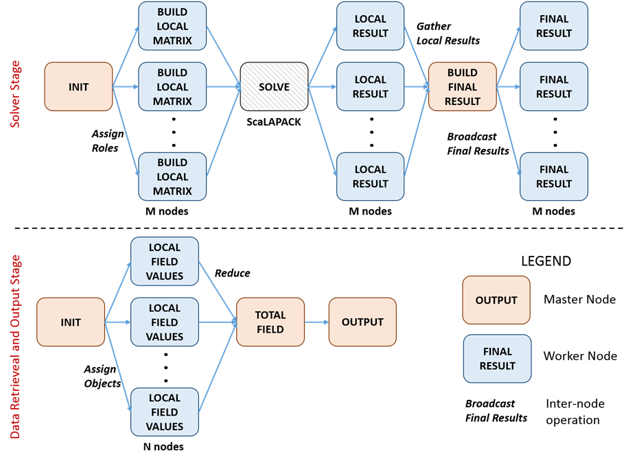
Figure
7. Inter-node communication scheme. Note that
after the scattering and internal field coefficients are calculated and stored,
the system is essentially “reset” and the next phase is independent of the
previous mapping. The example here is for a cluster with N particles, which are
initially mapped to M nodes. The final result will be an electromagnetic field
profile.
The inter-node
communication processes of OPTIMET-3D are illustrated in Fig. 7. In what
follows, we give a brief description of these processes. After the Master node initialises the simulation and chooses the appropriate
parallelisation strategy, the Worker nodes
are each assigned a piece of the scattering matrix to be build, i.e, a part of ![]() or
or
![]() . Each Worker
builds independently its assigned piece of the matrix. The first
. Each Worker
builds independently its assigned piece of the matrix. The first ![]() nodes,
nodes, ![]() being the number of particles in the system,
are then assigned the system matrix
being the number of particles in the system,
are then assigned the system matrix ![]() or
or ![]() , at which point ScaLAPACK is called to
solve the scattering matrix equation. Finally, the Master
node gathers the individual results from each of the
, at which point ScaLAPACK is called to
solve the scattering matrix equation. Finally, the Master
node gathers the individual results from each of the ![]() nodes and builds the solution vector containing the
Fourier expansion coefficients of the scattered field. The Master
node also calculates the internal field coefficients for each particle. This
last step can also be computed in parallel; however, numerical tests have shown
it to be of a reduced computational cost. Thus, in order to keep the inter-node
communication to a minimum, this operation is performed on the Master node only. Finally, the Master
node updates the Geometry object to include the newly computed internal
coefficients, which then broadcasts both the internal coefficients and the
solution vector to the remaining
nodes and builds the solution vector containing the
Fourier expansion coefficients of the scattered field. The Master
node also calculates the internal field coefficients for each particle. This
last step can also be computed in parallel; however, numerical tests have shown
it to be of a reduced computational cost. Thus, in order to keep the inter-node
communication to a minimum, this operation is performed on the Master node only. Finally, the Master
node updates the Geometry object to include the newly computed internal
coefficients, which then broadcasts both the internal coefficients and the
solution vector to the remaining ![]() nodes.
nodes.
At this point, the nodes
are ready to perform all other calculations that the user has requested. For
the field profile, for example, each node calculates the contribution from its
own assigned object and then the Master performs
a reduce operation in order to retrieve the total field on the grid. As the
field point locations are independent, more than ![]() nodes can be used for this computation, where
the individual grid points for each node to compute are selected. In the case
of a wavelength scan, for example, each node is assigned a portion of the
spectrum for which it calculates the far- and/or near-field responses. Each node
can then individually output the result to a single HDF5 file by using the
parallel output system, which is implicitly implemented by HDF5. It is
reiterated that no race condition occurs and that the load balancing is ensured
by enforcing that
each node is assigned to compute an equal work load from the desired spectrum
of frequencies.
nodes can be used for this computation, where
the individual grid points for each node to compute are selected. In the case
of a wavelength scan, for example, each node is assigned a portion of the
spectrum for which it calculates the far- and/or near-field responses. Each node
can then individually output the result to a single HDF5 file by using the
parallel output system, which is implicitly implemented by HDF5. It is
reiterated that no race condition occurs and that the load balancing is ensured
by enforcing that
each node is assigned to compute an equal work load from the desired spectrum
of frequencies.
For the non-linear
response calculations, a parallelisation strategy similar to the one employed
in the linear case is used. However, in this case each node needs to communicate
the corresponding non-linear source terms of their assigned particle(s) to all
the other nodes. The Master process
does not require any additional information to compute the non-linear response
because once the non-linear scattering coefficients are known,
the formalism is identical to that of the linear response calculations.
The parallelisation tasks
in OPTIMET-3D are provided via MPI. The
mathematical computations (i.e. linear
algebra operations), which require parallelisation are implemented through ScaLAPACK. In this particular case, all associated
inter-process communications are invoked by BLACS, which provides a very cost
effective interface for transferring among the nodes all data required. In this
implementation, ScaLAPACK and BLACS are chosen
because they are provided as the standard implementation of parallel algebra
computations in all major mathematical library distributions, including Intel’s
MKL and IBM’s ESSL. In addition, both packages are freely available from the netlib repository.
Finally, it should be
mentioned that we have also explored briefly the possibility of porting
OPTIMET-3D onto GPU-based clusters, such as nVidia’s Fermi architecture. Preliminary
investigations have shown that this code development would be very attractive,
both due to the enhancement of the functionality of the software, and, equally
important, because of the increase in the deployment base and potential of the
software.
6. Performance and Scalability Analysis
As presented in the
previous section, due to the high degree of parallelisability of the MSM
algorithm OPTIMET-3D is expected to perform very well when ported onto a
parallel computing environment. We have performed several performance tests for
the level of mapping, ![]() , using a series of clusters of spherical particles. The number of particles in the
cluster was
, using a series of clusters of spherical particles. The number of particles in the
cluster was ![]() The output data was the field profile on a
The output data was the field profile on a ![]() grid section located at the centre of the
cluster but outside of any of the spheres. This was done in order to ensure
that the actual performance data was related to the solver and not to any I/O
processes. In addition, the strong scalability of the parallelised OPTIMET-3D
solver was tested for the case of
grid section located at the centre of the
cluster but outside of any of the spheres. This was done in order to ensure
that the actual performance data was related to the solver and not to any I/O
processes. In addition, the strong scalability of the parallelised OPTIMET-3D
solver was tested for the case of ![]() .
.
6.1 Performance
Analysis
The focus of this section is the investigation of the
parallelised branch of OPTIMET-3D when different mapping levels, Lm, and corresponding number of nodes, ![]() are used. In Sec. 5.3, it was explained that
different Lm schemes would lead to different
resource usage conditions. In particular, it was concluded that the number of
processing nodes required,
are used. In Sec. 5.3, it was explained that
different Lm schemes would lead to different
resource usage conditions. In particular, it was concluded that the number of
processing nodes required, ![]() decreases as Lm
increases. Moreover, when one considers modern HPC systems, where the
associated memory available is typically below 4 GB per
decreases as Lm
increases. Moreover, when one considers modern HPC systems, where the
associated memory available is typically below 4 GB per ![]() , our tests have demonstrated that L3 is
an optimal choice. However, L2 can also be used efficiently in conjunction with
the edge mapping strategy, if all possible distribution scenarios can be
accounted for. Finally, L1 mapping is the most efficient mapping strategy in
terms of total execution time,
, our tests have demonstrated that L3 is
an optimal choice. However, L2 can also be used efficiently in conjunction with
the edge mapping strategy, if all possible distribution scenarios can be
accounted for. Finally, L1 mapping is the most efficient mapping strategy in
terms of total execution time, ![]() ; however, this is achieved at the
expense of a larger number
; however, this is achieved at the
expense of a larger number ![]() of
nodes being used. Thus, one has to bear in mind this trade-off when
using L1, as overall it could be regarded as being the least cost effective of
all schemes. In all simulations performed in this
work,
of
nodes being used. Thus, one has to bear in mind this trade-off when
using L1, as overall it could be regarded as being the least cost effective of
all schemes. In all simulations performed in this
work, ![]() includes both the computation time and
communication time.
includes both the computation time and
communication time.
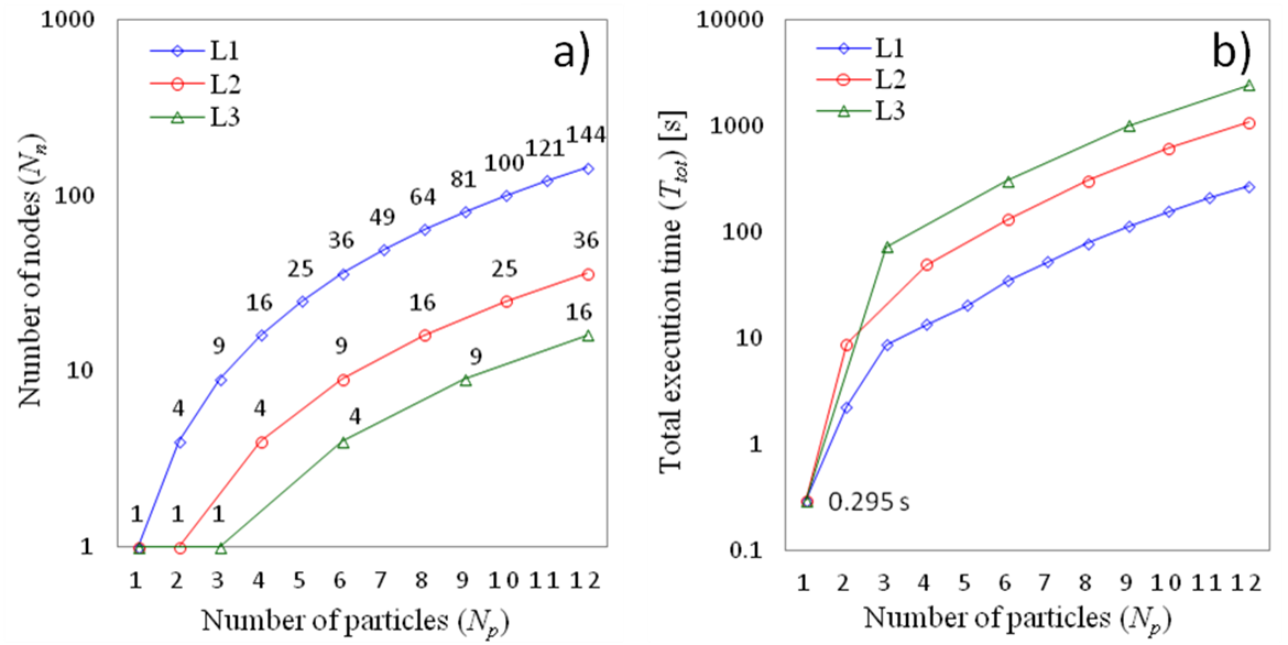
Figure 8. a)
Number of required nodes, ![]() vs. the number of particles,
vs. the number of particles,
![]() , for
three mapping levels, L1, L2 and L3.
, for
three mapping levels, L1, L2 and L3.![]() . b)
Total execution time,
. b)
Total execution time, ![]() , vs.
, vs. ![]() , for
the same mapping levels, L1, L2 and L3.
, for
the same mapping levels, L1, L2 and L3.
In order to illustrate
how the number of required computing nodes, ![]() , scale with the number of particles in
the cluster,
, scale with the number of particles in
the cluster, ![]() , we plot in Fig. 8(a) the dependence
, we plot in Fig. 8(a) the dependence![]() for three mapping orders,
for three mapping orders, ![]() . The cluster size is characterised by
the number of spheres,
. The cluster size is characterised by
the number of spheres, ![]() . For the case with
. For the case with ![]() particles, it is observed that the L1 strategy
requires
particles, it is observed that the L1 strategy
requires ![]() nodes, whilst
nodes, whilst ![]() decreases to
decreases to ![]() and
and ![]() for the L2 and L3 schemes, respectively.
for the L2 and L3 schemes, respectively.
In terms of the total
execution time, ![]() , we have run the test cases detailed
above, as per Fig. 8(b), on the Legion
cluster at UCL. The number of harmonics used was
, we have run the test cases detailed
above, as per Fig. 8(b), on the Legion
cluster at UCL. The number of harmonics used was ![]() which provides a typical value for simulations
of average complexity. We would expect that in most cases
which provides a typical value for simulations
of average complexity. We would expect that in most cases ![]() ranges from
ranges from ![]() if
dielectric particles are considered to
if
dielectric particles are considered to ![]() in
the case of metallic particles. In the latter case a larger
in
the case of metallic particles. In the latter case a larger ![]() is
required both due to increased permittivity of metals and the excitation of
strong optical resonances. As expected, L1 mapping level offers the lowest execution time, for example, for the cluster with
is
required both due to increased permittivity of metals and the excitation of
strong optical resonances. As expected, L1 mapping level offers the lowest execution time, for example, for the cluster with ![]() spheres,
spheres, ![]() . L3, on the other hand, shows on average
a 9 fold increase of the same simulation, namely, for
. L3, on the other hand, shows on average
a 9 fold increase of the same simulation, namely, for ![]() ,
, ![]() . This result is explained by the fact
that for
. This result is explained by the fact
that for ![]() , L3 scheme employs only
, L3 scheme employs only ![]() nodes, as opposed to the L1 schemes, which
requires
nodes, as opposed to the L1 schemes, which
requires ![]() nodes. It can be seen that the decrease in the
number of required nodes is exactly equal to 9. It should be noted that the small
discrepancies are attributable to non-uniform execution times due to ScaLAPACK’s speed improvements, which are found to slightly
depend on the particular content of the scattering matrix and the associated
inter-node communication costs.
nodes. It can be seen that the decrease in the
number of required nodes is exactly equal to 9. It should be noted that the small
discrepancies are attributable to non-uniform execution times due to ScaLAPACK’s speed improvements, which are found to slightly
depend on the particular content of the scattering matrix and the associated
inter-node communication costs.
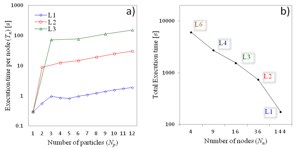
Figure 9. a)
Execution time per node, ![]() , vs.
the number of particles,
, vs.
the number of particles, ![]() , for
the case considered in Fig. 8, with three mapping levels,
, for
the case considered in Fig. 8, with three mapping levels, ![]() . b)
Strong scalability trend for a cluster of
. b)
Strong scalability trend for a cluster of ![]() =12
particles simulated with parallel mapping levels
=12
particles simulated with parallel mapping levels ![]() corresponding
to
corresponding
to ![]() =4, 9,
16, 36, 144 nodes,
respectively.
=4, 9,
16, 36, 144 nodes,
respectively.
For a more in-depth analysis of the performance of
OPTIMET-3D, the examination of the per node execution
time, ![]() , is considered
as shown in Fig. 9(a). This analysis clearly demonstrates that as one moves
from the serial code execution corresponding to the single-sphere problem (and
therefore from single-node execution) to the parallel branch of the software,
one observes a steep increase in the corresponding per node execution time,
, is considered
as shown in Fig. 9(a). This analysis clearly demonstrates that as one moves
from the serial code execution corresponding to the single-sphere problem (and
therefore from single-node execution) to the parallel branch of the software,
one observes a steep increase in the corresponding per node execution time, ![]() . In addition, this increase in
. In addition, this increase in ![]() is
considerably larger in the case of L3 scheme as compared to those of L2 and L1
levels. This is attributed to the fact that, for the cases studied here, the
total simulation time for the serial case is about
is
considerably larger in the case of L3 scheme as compared to those of L2 and L1
levels. This is attributed to the fact that, for the cases studied here, the
total simulation time for the serial case is about ![]() , namely, the communication costs greatly
dominate over the computation time. Moreover, as the mapping level increases,
the number of required nodes
, namely, the communication costs greatly
dominate over the computation time. Moreover, as the mapping level increases,
the number of required nodes ![]() decreases, and therefore the size of the
message per communication also increases. Therefore,
it is expected to observe a higher increase in
decreases, and therefore the size of the
message per communication also increases. Therefore,
it is expected to observe a higher increase in ![]() as
as
![]() increases, as in fact Fig. 9(a) illustrates.
It should also be noted that the L1 scheme was characterised by a smaller
increase in
increases, as in fact Fig. 9(a) illustrates.
It should also be noted that the L1 scheme was characterised by a smaller
increase in ![]() for an arbitrary
for an arbitrary![]() . This suggests that the L1 scheme
provides the fastest and most uniform CPU performance when compared to
. This suggests that the L1 scheme
provides the fastest and most uniform CPU performance when compared to ![]() . Nevertheless, this is achieved at the
expense of an increased
. Nevertheless, this is achieved at the
expense of an increased ![]() , which is regarded as a drawback of
using only L1. Thus, OPTIMET-3D offers great flexibility in the levels of
achievable parallelisation, as seen suitable by the user, based on the desired
simulation and hardware availability.
, which is regarded as a drawback of
using only L1. Thus, OPTIMET-3D offers great flexibility in the levels of
achievable parallelisation, as seen suitable by the user, based on the desired
simulation and hardware availability.
6.2 Scalability
Analysis
In this section, the strong scalability of the
parallelised branch of OPTIMET-3D is demonstrated. For this, we consider a
fixed problem size, ![]() , and measure the required
computation time corresponding to increasingly larger number of nodes,
, and measure the required
computation time corresponding to increasingly larger number of nodes, ![]() . Because of the particular
characteristics of OPTIMET-3D’s parallel mapping schemes, the number of
associated processing nodes,
. Because of the particular
characteristics of OPTIMET-3D’s parallel mapping schemes, the number of
associated processing nodes, ![]() , is determined by the level of mapping applied,
, is determined by the level of mapping applied, ![]() . In this test, we chose
. In this test, we chose
![]() , which resulted in
, which resulted in ![]() = {4, 9, 16, 36, 144} processes,
respectively. Constrained by the per node memory limitations of the available
HPC clusters (e.g., each node on the Legion cluster can access only 4 GB of RAM), in this study
we limited the number of angular harmonics to
= {4, 9, 16, 36, 144} processes,
respectively. Constrained by the per node memory limitations of the available
HPC clusters (e.g., each node on the Legion cluster can access only 4 GB of RAM), in this study
we limited the number of angular harmonics to ![]() , thus allowing for the L6 test case. It
should be noted that this relatively small value of
, thus allowing for the L6 test case. It
should be noted that this relatively small value of ![]() has a very limited influence on the overall
scalability of the parallelised solver. Moreover, the use of
has a very limited influence on the overall
scalability of the parallelised solver. Moreover, the use of ![]() is
usually well suited for cases in which the electromagnetic field is not too
spatially inhomogeneous, such as clusters of large dielectric particles
separated by distances of around 1/10 the size of the operating wavelength. In
cases where higher precision requirements are needed, the user can use the L4
or L3 mapping levels.
is
usually well suited for cases in which the electromagnetic field is not too
spatially inhomogeneous, such as clusters of large dielectric particles
separated by distances of around 1/10 the size of the operating wavelength. In
cases where higher precision requirements are needed, the user can use the L4
or L3 mapping levels.
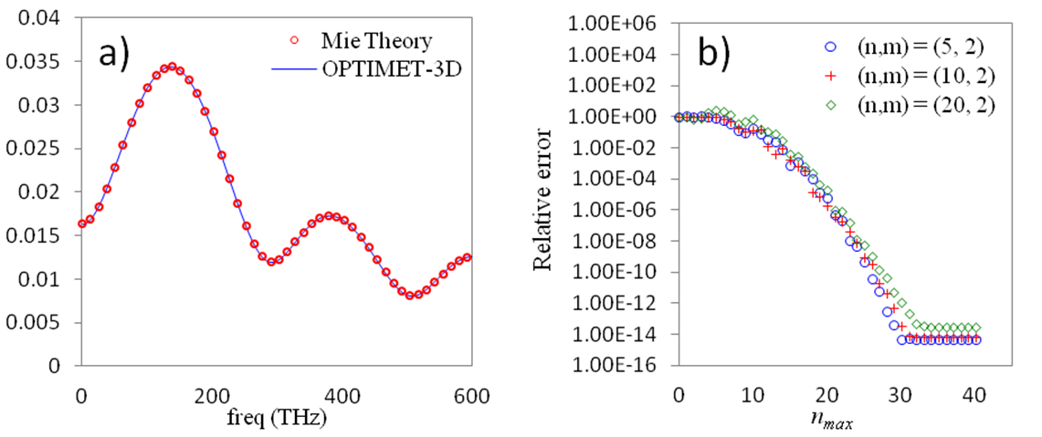
Figure 10. a) ![]() computed using
OPTIMET-3D solver and the Mie analytical solution for the single-particle
(sphere) problem. b) VSWFs translation-addition relative error vs. truncation
limit,
computed using
OPTIMET-3D solver and the Mie analytical solution for the single-particle
(sphere) problem. b) VSWFs translation-addition relative error vs. truncation
limit, ![]() .
.
The strong scalability of
the parallel branch of OPTIMET-3D is clearly demonstrated by the plots in Fig.
9(b). The linear reduction in the total execution time as the order ![]() of
the parallelisation level is reduced (i.e., number of
nodes is increased) is a direct consequence of the nature of the employed
parallelisation mappings, as well as the way in which the corresponding levels
evenly balance out all of the additional work load and related inter-process
communication. The higher mapping levels require fewer nodes, thus, they
require less inter-node communication. On the other hand, the work load
distributed to each node has now increased. This is clearly demonstrated when
comparing the total execution time as
of
the parallelisation level is reduced (i.e., number of
nodes is increased) is a direct consequence of the nature of the employed
parallelisation mappings, as well as the way in which the corresponding levels
evenly balance out all of the additional work load and related inter-process
communication. The higher mapping levels require fewer nodes, thus, they
require less inter-node communication. On the other hand, the work load
distributed to each node has now increased. This is clearly demonstrated when
comparing the total execution time as ![]() increases, where the per node computation time
dominates over the communication costs. In fact, even for lower Lm, where the contribution of inter-node communications
becomes more important, the strong scalability still holds. To conclude, the
OPTIMET-3D software demonstrates an excellent parallel performance, where
various mapping levels can be applied with similar effectiveness, thus,
allowing the user to target a desired execution time.
increases, where the per node computation time
dominates over the communication costs. In fact, even for lower Lm, where the contribution of inter-node communications
becomes more important, the strong scalability still holds. To conclude, the
OPTIMET-3D software demonstrates an excellent parallel performance, where
various mapping levels can be applied with similar effectiveness, thus,
allowing the user to target a desired execution time.
7. Code Validation and Practical Examples
In this section we present the results of a few tests we
performed in order to validate the code implementation and give an example of a
scientific problem that OPTIMET-3D can be used to investigate. Thus, we first
examine the electromagnetic wave scattering from a sphere and compare
analytical results based on Mie theory with those obtained using OPTIMET-3D.
Then, we show the results of some numerical experiments illustrating
convergence of the translated VSWFs, which are used throughout the code.
Finally, we illustrate how OPTIMET-3D can be used to investigate a nano-photonics problem, namely, light scattering from a
dimer and chiral clusters of silicon nano-spheres.
7.1 Single Particle Problem - Sphere
Consider a homogeneous
sphere of radius ![]() , made of nonmagnetic, lossless and
non-dispersive material with relative permittivity
, made of nonmagnetic, lossless and
non-dispersive material with relative permittivity ![]() , embedded in a homogeneous medium with
, embedded in a homogeneous medium with ![]() and
and
![]() . The sphere is excited with a
monochromatic electromagnetic plane wave with frequency,
. The sphere is excited with a
monochromatic electromagnetic plane wave with frequency,![]() . The scattered electric field,
. The scattered electric field,![]() ,
, ![]() , is calculated using OPTIMET-3D and the
analytical formalism based on the Mie theory [2]. The field
, is calculated using OPTIMET-3D and the
analytical formalism based on the Mie theory [2]. The field ![]() calculated by using these two methods is
plotted in Fig. 10(a). These results clearly demonstrate the accuracy with
which OPTIMET-3D can perform these field calculations.
calculated by using these two methods is
plotted in Fig. 10(a). These results clearly demonstrate the accuracy with
which OPTIMET-3D can perform these field calculations.
7.2 Validation of code implementation of the
Vector Translation-Addition Theorem
At the heart of the MSM
algorithm is the ability to translate incoming and outgoing VSWFs, expressed in
the co-ordinate system with origin in ![]() , to a co-ordinate system with origin in
, to a co-ordinate system with origin in ![]() . This is achieved by using the vector translation-addition theorem:
. This is achieved by using the vector translation-addition theorem:
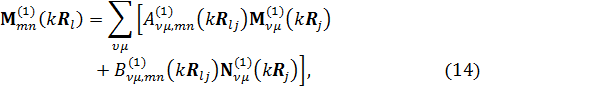
where ![]() and
and ![]() ,
, ![]() , represent the vector
translation-addition coefficients [2, 4]. In order to illustrate the validity
of our computer implementation of these relations, we plot in Fig. 10(b) the
relative error as function of the truncation limit used in calculating the sum
in Eq. (14),
, represent the vector
translation-addition coefficients [2, 4]. In order to illustrate the validity
of our computer implementation of these relations, we plot in Fig. 10(b) the
relative error as function of the truncation limit used in calculating the sum
in Eq. (14), ![]() , for a translation distance
, for a translation distance ![]() ,
,![]() , and
, and ![]() . Note that such convergence tests are extremely useful
in assessing the size of particle clusters that can be modelled with
OPTIMET-3D, as well as the number of harmonics that one must include to study
clusters of particles made of specific materials. This information, in turn,
will be used when the Balancer class will be fully implemented.
. Note that such convergence tests are extremely useful
in assessing the size of particle clusters that can be modelled with
OPTIMET-3D, as well as the number of harmonics that one must include to study
clusters of particles made of specific materials. This information, in turn,
will be used when the Balancer class will be fully implemented.
7.3 Two Particles Problem – Dimer
In a more complex test,
we calculated the spatial distribution of the electromagnetic field scattered
by two dielectric spheres made of silicon, at both the FF and SH. This allowed
us to test both the linear and non-linear branches of OPTIMET-3D. The results
are plotted in Fig. 11. As expected, the field profile at the FF has a
symmetric scattering pattern that suggests the interference between the
incoming and scattered waves, whereas at the SH the field originates at the
surface of the two spheres made of silicon. The field profiles in Fig. 11 also
show the field discontinuities at the surface of the two spheres, which
illustrates that the boundary conditions are properly incorporated in the code.
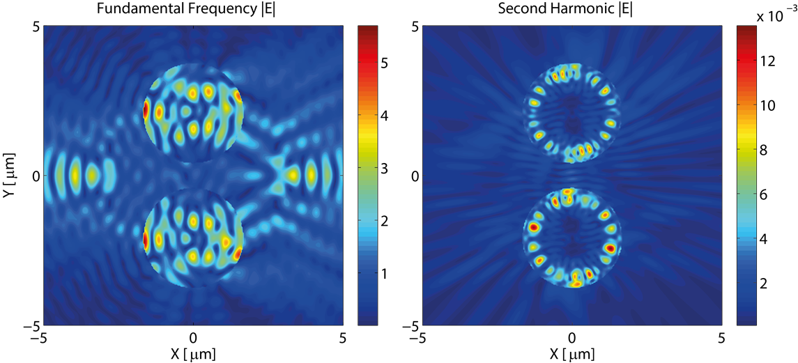
Figure 11. Field profile at FF (left) and SH (right), respectively, generated
by scattering from two silicon spheres.
7.4 Super-Chirality from a Cluster of
Dielectric Nano-Spheres
As an example of how OPTIMET-3D is used to study a
problem of practical importance, we present in this section the results of a
few simulations pertaining to light interaction with a chiral nano-optical structure. In particular, we demonstrate that the scattered
optical field of photonic nanostructures with intrinsic chirality, which are
made of silicon spheres, exhibits strong optical chirality as well as enhanced
circular differential scattering. In addition, this analysis shows that using
such resonant chiral nanostructures allows one to easily achieve super-chiral
optical fields whose optical chirality is more than two orders of magnitude
larger than that of circularly polarised plane waves.
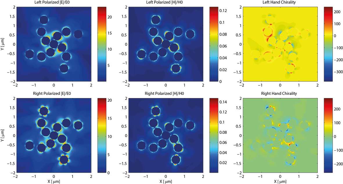
Figure 12. Electromagnetic field distribution and optical chirality of the
scattered field of a chiral nano-sphere cluster for
left- (top panels) and right- (bottom panels) circularly polarised light.
The nano-cluster consists
of silicon spheres with radius  , arranged in a chiral pattern.
The cluster is excited by a circularly polarized plane wave with wavelength,
, arranged in a chiral pattern.
The cluster is excited by a circularly polarized plane wave with wavelength,  , which is chosen to coincide
with one of the optical resonances (TE mode) of the spheres. The optical
resonances are determined by computing the spectrum
of the field enhancement at an arbitrary position near one of the spheres, as
indicated in Fig. 12. The chirality of the optical field,
, which is chosen to coincide
with one of the optical resonances (TE mode) of the spheres. The optical
resonances are determined by computing the spectrum
of the field enhancement at an arbitrary position near one of the spheres, as
indicated in Fig. 12. The chirality of the optical field,  , can be calculated once the
field distribution is known. For super-chiral fields,
, can be calculated once the
field distribution is known. For super-chiral fields, . Our analysis
shows that the chirality of the optical field is strongly enhanced at the
resonance wavelength when the cluster is perpendicularly illuminated by
circularly polarized plane waves, the field being highly super-chiral in large
domains. In particular, more than two orders of magnitude enhancement of the
chirality is observed. Importantly, the chirality of the optical near-field
also indicates a strong circular differential scattering of the chiral cluster
we investigated.
. Our analysis
shows that the chirality of the optical field is strongly enhanced at the
resonance wavelength when the cluster is perpendicularly illuminated by
circularly polarized plane waves, the field being highly super-chiral in large
domains. In particular, more than two orders of magnitude enhancement of the
chirality is observed. Importantly, the chirality of the optical near-field
also indicates a strong circular differential scattering of the chiral cluster
we investigated.
8.
Project Impact
The main aim of this project, which has been fully accomplished,
was to develop an open source HPC software to be used
on UCL's HPC main system, Legion. Because
of its portability and easy to use features, OPTIMET-3D can be easily installed
and used on HPC systems with different configurations. The software was
designed to model both the linear and non-linear interaction of electromagnetic
waves with arbitrary distributions of 2D and 3D particles. In the 3D case one can impose periodic boundary
conditions, which enhances the spectrum of science and engineering problems
that can be studied. Equally important, the range of materials that can be
described by OPTIMET-3D covers most cases of practical interest, including,
metals, dielectrics, polaritonic materials and
semiconductors.
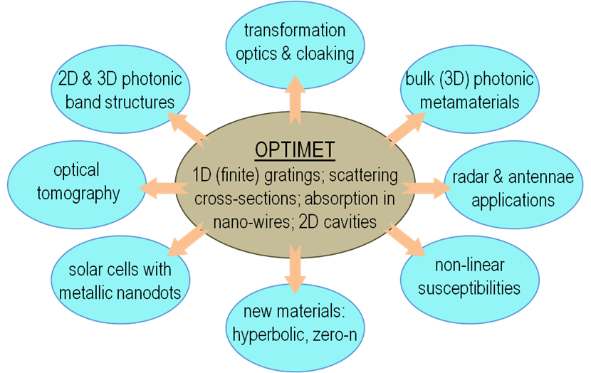
Figure
13.
By extending OPTIMET to OPTIMET-3D the applications space has increased
dramatically.
As illustrated in Fig. 13, by
extending OPTIMET to 3D structures we have dramatically increased the spectrum
of science and engineering problems that we can investigate. Thus, to outline
just a few of its features important for practical applications, OPTIMET-3D can
now be used to investigate linear and non-linear optical properties of
realistic, 3D photonic systems and devices, which are randomly or periodically
structured, it can be used to compute effective linear and non-linear optical
constants, such as effective permittivity and effective non-linear
susceptibilities of metamaterials and it can be used
to calculate the optical absorption in systems of particles. These
functionalities make OPTIMET-3D extremely useful in studying a series of
problems pertaining to linear and non-linear photonic and plasmonic
crystals, absorption engineering (with applications to solar cells and other
photovoltaic devices), transformation optics, optical tomography, colloidal
chemistry and many others.
We intend to use
OPTIMET-3D in a series of research projects, as part of ongoing
collaborations and new ones. A brief outline of such projects is presented in
what follows.
·
We plan to use OPTIMET-3D to study the non-linear
optical properties of non-linear plasmonic metamaterials (in collaboration with Dr Paul Warburton’s
Group at UCL).
·
We will use OPTIMET-3D to study the
absorption/emission properties of molecules placed at nanometre distance from
metallic nano-particles (in collaboration with Prof
Richard Osgood’s Group at Columbia University). This work is particularly
relevant to the design of next-generation solar cells that incorporate plasmonic materials.
·
In collaboration with Prof Jeremy Baumberg
and Dr Ventsislav Valev
(University of Cambridge) we will use OPTIMET-3D to interpret experimental data
regarding optical properties of self-assembled clusters of metallic nano-particles.
·
We will use OPTIMET-3D to study multi-colour Anderson
wave localisation in disordered ensembles of dielectric nano-particles
(in collaboration with Prof Chee Wei Wong's Group at
Columbia University).
·
We will use OPTIMET-3D to study optical properties of quantum
meta-materials, a project supported by EPSRC/NSF (EP/J018473/1) (in
collaboration with Prof Shuang Zhang's Group at the
University of Birmingham and Prof Xiang Zhang's Group at Berkeley University).
9.
Conclusions and Future Work
In this report we have described
the structure, code implementation (parallel and serial), validation tests and
a few application examples of OPTIMET-3D. This HPC software package
has been developed with support from EPSRC's University
distributed Computational Science and
Engineering (dCSE) Programme.
OPTIMET-3D has been written and tested for validity and scalability, as
illustrated in this report, with strong scalability being proven. It can be
used to model a broad array of science and engineering problems, including
photonic and plasmonic crystals, absorption
engineering, nanoscience and nanotechnology, plasmonics, transformation optics, optical tomography and
colloidal chemistry.
The HPC code has been developed
for Legion, UCL's main HPC cluster, but has
been tested on two other HPC systems, the InfraGrid
and BlueGene/P clusters at the West University of
Timisoara. The fully verified and tested code will be made available through
the BitBucket
website, a dedicated webpage at UCL and through the program library of Computer
Physics Communications journal via a
peer-reviewed journal article. The uni-dCSE support
was for 12 months FTE divided between two people, Dr Ahmed Al-Jarro and Dr Claudiu Biris. A conference paper based on OPTIMET-3D will be
presented shortly after the project has ended [6].
In order to further advance the
functional capabilities of OPTIMET-3D, while building on the success of this
initial project, we plan a set of future code development activities.
·
We plan to port
OPTIMET-3D on massively parallel architectures, including UK's HECToR and ARCHER, the next national HPC
facility for academic research.
For this, subsequent uni-dCSE projects, when called
for, or future dCSE support will be sought.
·
We will explore the portability of OPTIMET-3D
to
multi-GPU HPC clusters (one such cluster is available at UCL).
·
We plan to make
OPTIMET-3D the electromagnetic solver, which when combined with a quantum
mechanical solver, will provide the unique functionality of modelling hybrid
classical/quantum mechanical physical systems [13-15].
·
We will
implement the dynamical Balancer
described in Sec. 5, which will help distribute among the nodes the work load
in a more balanced way.
·
We will
implement the hybrid mapping scheme for parallelisation, which could prove to
be more effective in both balancing the work load among the nodes and offering
the highest flexibility in the available computing resource.
·
In order to make
the code easier to use, we plan to add a GUI that would allow graphical input
of the simulation parameters. Note that since we use XML standards, such a GUI
could be easily adapted from existing XML editors.
Acknowledgement
This
project was funded under the HECToR Distributed
Computational Science and Engineering (CSE) Service operated by NAG Ltd. HECToR – A Research Councils UK High End Computing Service
– is the UK's national supercomputing service, managed by EPSRC on behalf of
the participating Research Councils. Its mission is to support capability
science and engineering in UK academia. The HECToR
supercomputers are managed by UoE HPCx
Ltd and the CSE Support Service is provided by NAG Ltd.
http://www.hector.ac.uk.
References
[1] C. F. Bohren and D. R. Huffman, Absorption
and Scattering of Light by Small Particles, (Wiley-Interscience, 1983).
[2] M. Mishchenko,
L. Travis, and A. Laci, Scattering,
Absorption and Emission of Light by Small Particles, (Cambridge
University Press 2002).
[3] M. I. Mishchenkoa, G. Videenb, V. A. Babenkoc, N. G. Khlebtsovd, and
T. Wriedt, “Comprehensive T-matrix
reference database: A 2004–06 update,” J. Quant. Spectr. Rad. Trans. 106, 304–324
(2007).
[4] B. Stout, J.-C.
Auger, and J. Lafait, “A transfer
matrix approach to local field calculations in multiple scattering problems,” J. Mod. Opt. 49, 2129–2152 (2002).
[5] C. G. Biris and N. C. Panoiu, “Second harmonic generation in metamaterials
based on homogenous centrosymmetric nanowires,”
Phys. Rev. B, 81, 195102 (2010).
[6] C. G. Biris, A. Al-Jarro, and N. C. Panoiu, “Super-chiral Effects in
Silicon Nano-sphere Clusters,” Proceedings of the 34
Progress in Electromagnetics Research (PIERS), Stockholm, Sweden, Aug. 12-15
(2013).
[7] A. Capretti, C.
Forestiere, L. D. Negro, and G. Miano,
“Full-wave analytical solution of second-harmonic
generation in metal nanospheres”, arXive, 2013.
[8] T. Heinz, “Second-order
nonlinear optical effects at surfaces and interfaces,” in Nonlinear surface
electromagnetic phenomena, Modern problems in condensed matter sciences,
edited by H. Ponath and G. Stegeman,
pp. 353–416 (1991).
[9] M. Lax, “Multiple
scattering of waves,” Rev. Mod. Phys. 23, 287–310 (1951).
[10]
N. Stefanou
and A. Modinos, “Scattering
of light from a two-dimensional array of spherical particles on a substrate,”
J. Phys.: Condens. Matter 3,
8135–8148 (1991).
[11]
N. Stefanou,
V. Karathanos, and A. Modinos, “Scattering
of electromagnetic waves from periodic structures,” J. Phys.: Condens. Matter 4, 7389–7400 (1992).
[12]
C. G. Biris and N. C. Panoiu, “Nonlinear pulsed excitation of high-Q optical modes
of plasmonic cavities made of metallic nanowires,” Opt. Express 18, 17165–17179 (2010).
[13]
M. Bahl,
N. C. Panoiu, and R. M. Osgood, “Optical and
thermal finite-difference time-domain model for passively mode-locked
surface-emitting lasers,” J. Opt. Soc. Am. B 26,
1558-1568 (2009).
[14]
H. Chen, J. M. McMahon, M.
A. Ratner, and G. C. Schatz, “Classical Electrodynamics
Coupled to Quantum Mechanics for Calculation of Molecular Optical Properties: a
RT-TDDFT/FDTD Approach,” J.
Phys. Chem. C 114, 14384-14392 (2010).
[15]
L. Pierantoni, D. Mencarelli,
and T. Rozzi, “A New 3-D Transmission Line Matrix Scheme
for the Combined Schrödinger–Maxwell Problem in the Electronic/Electromagnetic
Characterization of Nanodevices,” IEEE Trans.
Microwave Theor. Tech. 56,
654–662 (2008).