 |
Seismic wave calculation at the Hz level for a general Earth
Paul Roberts
Numerical Algorithms Group Ltd,
Wilkinson House, Jordan Hill Road, Oxford, OX2 8DR, UK,
Date: 31st June, 2013
This dCSE project will concern the attempt to improve the performance of a seismic wave propagation code, SPECFEM3D-GLOBE.
The original project plan was to become familiar with the code and then perform a series optimisations. Some runs were unstable, which required analysis of these cases to find the source of the defects and consequently improve the code so that it runs stably and more efficiently. This would be followed by merging two main sections of code into one, removing the need to write and read large temporary files to disk (up to at least 3 TB), boosting performance. Up to around 8% of the walltime of a calculation is taken up in mesh I/O, so removing this will achieve a speedup of the same value.
This project was approved for 5 months effort in June 2012 and was completed June 2013. The work was supervised by Dr James Wookey of the School of Earth Sciences at the University of Bristol with advice and assistance provided by Dr Andy Nowacki and Dr Andrew Walker both also from the School of Earth Sciences at the University of Bristol.Abstract:
The code which is the subject of this proposal, SPECFEM3D_GLOBE [1,2], simulates the propagation of seismic waves inside the Earth. It uses the spectral finite-element method and solves the acoustic-viscoelastic wave equation in the time domain. It allows the incorporation of the effects of gravity, attenuation, surface topography, and fully-general elastic structure in the mantle. Because it uses the spectral finite-element method (SEM), only one communication round between elements is required per time step [2], making it especially suitable for large-scale computing. It is written in ~ 71, 000 lines (~ 380 subroutines) of Fortran 95 with MPI for all communications, with two C routines for I/O and regular expression parsing. Apart from this, no libraries are required and the code is used on a wide variety of clusters and HPC facilities, including HECToR.
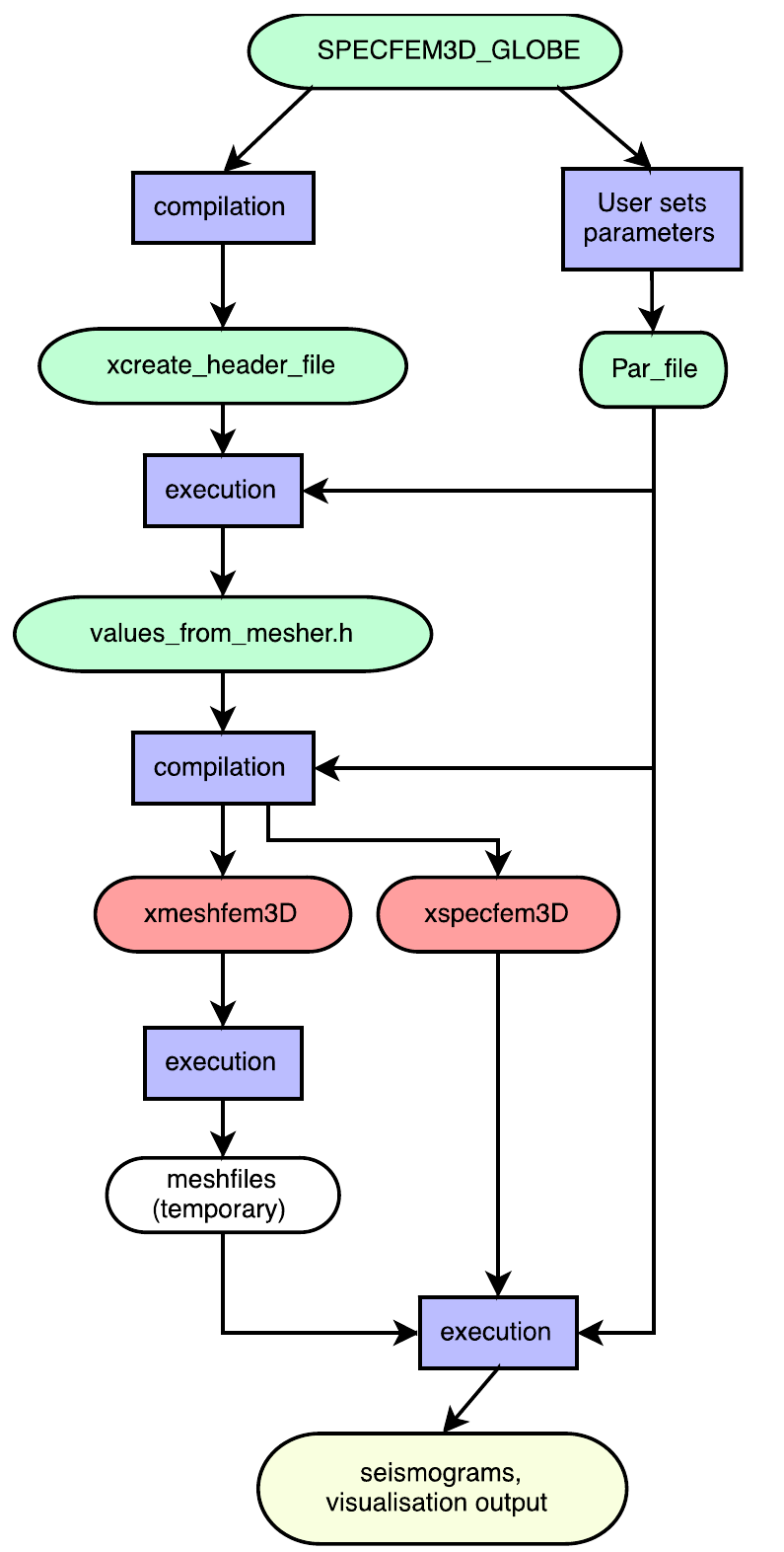
In its current form, the code must be run in two stages as two separate executables: (i) the SEM mesh is produced and mesh files written to disk; (ii) mesh files are read and the simulation is run, solving for the specified initial conditions. The first, meshing stage at present requires the seismic model to be described explicitly in the code, or as special subroutines written to read in data files in a specific format. The writing and reading of mesh files to disk means that some properties of the simulation can be changed and the solving stage run without having to re-mesh, but means several hundred GB of data and potentially tens of thousands of files must be written for practically every run. Despite using Fortran binary files, the time taken for I/O is often substantial (e.g., up to 8% of the total walltime). The code at present uses statically-allocated memory, requiring the code to be recompiled any time one of the parameters is changed (e.g., which seismic model is used), apart from some specific features (e.g., where to write output files). A Fortran 95 program (xcreate_header_file) computes the size of arrays needed in the two executables (the mesher, xmeshfem3D, and the solver, xspecfem3D) based on parameter choices, and writes a header file which is included in the compilation of the main executables. These are then run in sequence, both in parallel across the cluster or other HPC machine. Compilation is with the Cray compilers using the default level of optimisation with no additional specific optimisation flags. This workflow is represented in Figure 1.
The package can run either in single or in double precision mode with the default being single precision since, for almost all of the calculations performed using the spectral-element method, using single precision is sufficient and gives the same results (i.e. the same seismograms); and the single precision code is faster and requires significantly less memory.
This program takes user input and, according to the options set, builds a mesh for use by xspecfem3D to later solve the wave equation. It uses a series of subroutines for each Earth model to produce the elasticity in the region of interest (
![]() ,
,
![]() or the whole Earth), which might vary only radially (1D models) or fully in all dimensions (3D models). Further, the elasticity might be independent of direction (isotropic) or vary with direction (anisotropic).
or the whole Earth), which might vary only radially (1D models) or fully in all dimensions (3D models). Further, the elasticity might be independent of direction (isotropic) or vary with direction (anisotropic).
The mesher reads in user options regarding the seismic model, number of chunks and boundary conditions etc. from a parameter file Par_file, which resides in the subdirectory DATA.
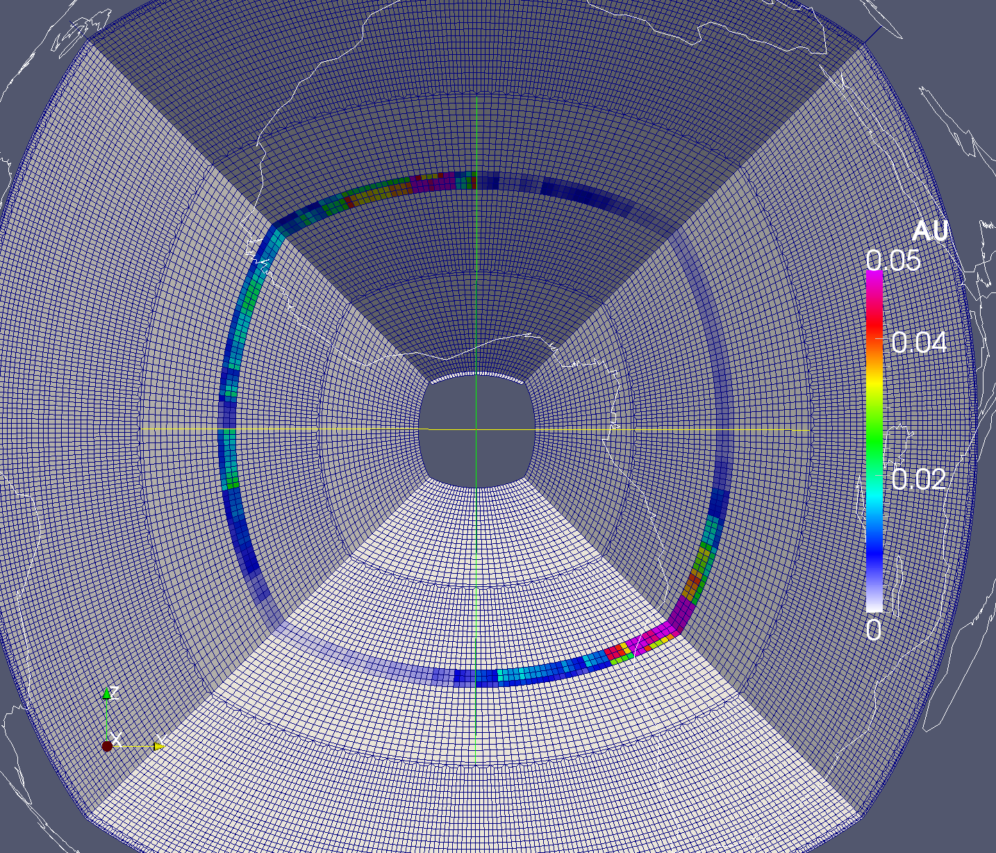
An example of the mesh is shown in Figure 2 where AU is a measure of the strength of anisotropy. Elsewhere in the model, the velocities are isotropic. This shows the sides of one of the two chunks of the mesh. The elements are shown by the outlines, and you can see the doubling of the mesh near the surface, in the mantle, and in the outer core. The inner core is absent from the mesh (you can see through the hole in the middle). Coastlines are shown as white lines.
The solver reads in the mesh produced by the mesher. It also reads in the user's options for the solver stage from three files:
Most current users of SPECFEM3D_GLOBE are interested in long-wavelength seismic phenomena, examining cases where the maximum frequency f is similar to 0.01 Hz and less. For such calculations, an existing empirical relationship between the frequency and maximum timestep of the calculation is employed to ensure stable calculations. However, many existing and potential users of the software are interested in shorter-wavelength features and would like to use the code at higher frequencies. In this case, no empirical stability criteria exist and there is limited experience of calculating high-frequency seismograms. Rigorous testing of the code's stability is necessary to ensure reliable performance. This may also involve finding bugs or over/underflow problems. Such instability is straightforward to identify, as displacements will become infinitely large and the program will exit with failure. Before the start of this DCSE project, Andy Nowacki has run SPECFEM3D_GLOBE on HECToR using up to 1350 cores for walltimes of 6 hours, performing simulations at ~ 0.05 - 0.1Hz.
The original proposal submitted to the dCSE panel requested 5 months effort. The original objectives for this project were as follows:
Work package 0: Code Familiarization (Effort: 0.5 month, Full time)
Two weeks will be spent becoming familiar with the code. The PIs will provide test simulations with benchmarked output for up to 864 cores (6.7M elements, 450M points) and these will be run with the unmodified code.
Runs will be monitored with graphical debugging tools to follow the flow of the programs.
Milestone 1: Successful run of test simulations provided by PIs.
Work package 1: Stability analysis, optimisation strategies and benchmarking. (Effort: 2 months, Full time)
Use debugging and profiling to improve the stability of the code for high-frequency calculations, and find optimal compiler configurations for use on HECToR.
Milestone 1: Successful run of test simulations provided by PIs.
Work package 2: Merging of mesher and solver stages. (Effort: 2 months, Full time)
Remove the disk I/O bottleneck in performance and disk usage. Currently, very large (up to 700GB) Fortran binary mesh files are produced, with disk I/O taking up to 8% of the total walltime. Each MPI process writes the part of the mesh it works on in parallel, where up to 50k processes may be used in the proposed work package.
The two executables (mesher and solver) will be merged into one so that no files need be written and read as an intermediate step. The separation of the two processes will be kept as a runtime option settable by the user.
Milestones 3 and 4: Working combined program with memory use similar to the separate programs.
Work package 3: Merging of updated code into development branch and Final Report. (Effort: 0.5 months, Full time)
To be produced in html and .pdf format ready for publication on the HECToR website. Status update on code being released to users.
The only changes to the original workplan were to run the project at 50% effort over 10 months.
On HECToR Phase 3, the compute and head nodes have a different architecture: the compute nodes have the newer AMD Interlagos processors, whilst the head nodes have the Istanbul type. This causes problems because xcreate_header_files is run on the head nodes at compile-time, and would by default be built for the compute nodes. Therefore one must either
${MODULESHOME}/init/sh  # This adds directories to your PATH
module swap xtpe-interlagos xtpe-istanbul  # Swap architecture
cd src/create_header_file; make            # Make for head nodes
module swap xtpe-istanbul xtpe-interlagos  # Swap back
However, the xcreate_header_file program requires many of the source files that are also used by the mesher and solver, so we additionally create a new directory for object files for linking into xcreate_header_file on the head nodes, obj_head_node.
The Cray Fortran compiler, crayftn, does not by default create .mod files for modules. We need them, so we need flag -em.
OpenMP can be used optionally in SPECFEM3D_GLOBE, but there's not a major performance boost on the XE6 because MPI calls within nodes are effective ly reduced to internal memory transfers. However, OpenMP flags are compiled in by default, so we need to turn them off with -h noomp.
When using the PrgEnv-cray module, CCE uses Google's tcmalloc library rather than the system malloc. This causes a problem somewhere during the configure stage as the configure script puts it in twice. Adding the flag -h system_alloc to the Cray compiler flags forces it back to the system malloc which pgi and gnu use and fixes the issue.
Initial attempts at profiling SPECFEM3D_GLOBE using CrayPAT were unsucessful due to what appears to be a bug in CrayPAT. The mesher runs to completion successfully but the solver hangs early on in the calculation when attempting to run a version instrumented with the pat_build command. Eventually Tom Edwards from Cray provided the following work around:
The problem appears to be that something in the MPI library is failing when the timer code interrupts the application during the sampling, however tracing experiments appear to be unaffected.
The following is a workaround for the application until the problem is properly resolved. It looks like the abort can be avoided by changing how the sampling occurs in the application. Instead of using regular timers to initiate samples as is the default with APA, it is possible to use hardware counter overflows as the trigger points for the sampling. The following environment variables attempt to sample at the same frequency (10000 microseconds) as normal but use the L1 Data Cache Misses at the trigger rather than wallclock time. We also have to change the type of experiment used to Program Counter at HWPC Overflow.
export PAT_RT_HWPC_OVERFLOW="PAPI_L1_DCM:10000s"
export PAT_RT_EXPERIMENT="samp_pc_ovfl"
This seems to be sufficient to collect effective statistics, but avoid the initial abort. My testing has shown that we can now generate an APA file for this application.
In the meantime Scalasca was an adequate alternative providing the required information on the most expensive subroutines.
To aid with portability we made the following changes, replacing
integer, parameter :: SIZE_REAL = 4, SIZE_DOUBLE = 8in the constants.h file with
integer, parameter :: SIZE_REAL=selected_real_kind(6)
integer, parameter :: SIZE_DOUBLE=selected_real_kind(12)
and then throughout the source code changed
real(kind=4)
DOUBLE PRECISION
sngl(foo)
to
real(kind=SIZE_REAL)
real(kind=SIZE_DOUBLE)
real(foo,kind=SIZE_REAL)
Significant effort has been spent on making this merged version of SPECFEM3D_GLOBE backwards compatible with the original separate mesher/solver paradigm. To this end we introduced 3 logical parameters WRITE_MESH, READ_MESH and JUST_SOLVE to the parameter file Par_file which control the behaviour of the new merged version of the code. We also added a dummy driving routine, meshfem3D_solo.f90, that is just a wrapper to the mesher so that it can be used separately and an interface to the mesher mesh_interfaces.f90 to give more compile time checking and because it's needed if you want to pass an unallocated variable in and out of a subroutine that then allocates it.
During the course of this DCSE project a number of bugs which affected the code's stability were discovered and fixed by the SPECFEM authors which were then merged into the CoMITAC version which is the version that the DCSE was improving.
Initial testing and benchmarking was performed using CCE, the Cray Compiling Environment, on a variety of problem sizes and types. These included regional simulations running the code in 1 or 2 chunk mode [1] and simulations at the scale of the entire globe which use 6 chunks and with or without Attenuation [3] turned on. This increases the memory requirements significantly (roughly by a factor of 2), and is numerically fairly expensive [1]. The build process uses the standard configure and make shell scripts and separates out the compiler flags via the following variables: FLAGS_CHECK - the compiler flags for the non-critical subroutines and FLAGS_NO_CHECK - the compiler flags for creating fast, production-run code for the critical subroutines. For some of the more testing examples provided there was a requirement for FLAGS_NO_CHECK to be set to -O0, that is with no optimisation, to prevent the runs becoming numerically unstable and fail with the error: "the forward simulation became unstable and blew up in the solid". This of course had an unacceptable effect on the performance of the code. Fortunately experimentation with the different compiler suites available on HECToR (including NAG, PGI and GNU) led us to discover that PGI could run the simulation that was previously failing with an optimisation level of -O3 -fast in both FLAGS_NO_CHECK and FLAGS_CHECK. However we then ran into issue raised by work package 2 as this generated over 1TB of mesh and using double precision generated output of over 2.5TB. This leads nicely into the next section.
Running SPECFEM3D_GLOBE involves running two separate executables - firstly the mesher, xmeshfem3d, which generates the mesh and writes it to disk with each process writing its own Fortran binary file. This is followed by running the solver xspecfem3d which reads in those files and then performs the required calculations. This can be advantagous since the solver can be rerun without having to rerun the mesher and for this reason we retain this functionality in our merged version of SPECFEM3D_GLOBE. Unfortunately the code uses statically-allocated memory, requiring the code to be recompiled any time one of the parameters is changed (e.g., which seismic model is used), apart from some specific features (e.g., where to write output files). A Fortran 95 program (xcreate_header_file) computes the size of arrays needed in the two executables (mesher, xmeshfem3D, and solver, xspecfem3D) based on parameter choices, and writes a header file which is included in the compilation of the solver.
On HECToR each of the meshers files has to be written to a globally mounted file system, LUSTRE, which can create a large bottleneck for both the mesher and the solver due to I/O contention. The original version of the code writes and reads up to 51 files per core. As mentioned in the previous section this can easily reach multiple terabytes of data which is therefore a major factor for large simulations.
This bottleneck has been removed by merging the mesher and solver into a single application through turning the mesher into a subroutine that is called by the solver and passing the data around rather than using I/O. Merging the codes was technically difficult because it brought challenges in memory management and name space pollution across the two originally separate applications. There was also the need to retain the original functionality of being able to separately run the mesher or solver (with the I/O intact) or indeed run both together but still write the mesh to disk. By setting the logical variables WRITE_MESH, READ_MESH and JUST_SOLVE in the Par_file and the use of the new driving routine meshfem3D_solo.f90 this has been acheived. It is currently a compile time choice which the program xcreate_header_file writes to the file values_from_mesher.h but there is the option to make it a run time choice in the future.
We were able to completely eliminate the need for I/O to communicate between the two parts of SPECFEM3D_GLOBE, removing the need to use any disk space for intermediate files along with the associated I/O penalties of using these files. The main problems we faced in performing the merge came from memory footprint since in the initial merged version some of the arrays from the mesher and from the solver had to be present in memory simultaneously. This was problematic because the more memory per core required, the more likely the need to underpopulate HECToR nodes when running the higher frequency simulations that are the goal. Which in turn means increase in AU cost. To reduce this memory usage we rewrote the mesher to use the arrays from the solver which in turn required separate calls to the approapriate subroutines.
For example, the original call to create_reigions_mesh looked like this
call create_regions_mesh(iregion_code,ibool,idoubling,is_on_a_slice_edge,&
  xstore,ystore,zstore,rmins,rmaxs,iproc_xi,iproc_eta,ichunk,&
  NSPEC(iregion_code),nspec_tiso,volume_local,area_local_bottom,&
  area_local_top,nglob(iregion_code),npointot,NSTEP,DT,NEX_XI,&
  NEX_PER_PROC_XI,NEX_PER_PROC_ETA,NSPEC2DMAX_XMIN_XMAX(iregion_code),&
  NSPEC2DMAX_YMIN_YMAX(iregion_code),NSPEC2D_BOTTOM(iregion_code),&
  NSPEC2D_TOP(iregion_code),NPROC_XI,NPROC_ETA,NSPEC2D_XI_FACE, &
  NSPEC2D_ETA_FACE,NSPEC1D_RADIAL_CORNER,NGLOB1D_RADIAL_CORNER,&
  myrank,LOCAL_PATH,rotation_matrix,ANGULAR_WIDTH_XI_RAD,
  ANGULAR_WIDTH_ETA_RAD,SAVE_MESH_FILES,NCHUNKS,INCLUDE_CENTRAL_CUBE,&
  ABSORBING_CONDITIONS,R_CENTRAL_CUBE,RICB,RHO_OCEANS,RCMB,R670,RMOHO,&
  RMOHO_FICTITIOUS_IN_MESHER,RTOPDDOUBLEPRIME,R600,R220,R771,R400,R120,&
  R80,RMIDDLE_CRUST,ROCEAN,ner,ratio_sampling_array,doubling_index,&
  r_bottom,r_top,this_region_has_a_doubling,ipass,&
  ratio_divide_central_cube, CUT_SUPERBRICK_XI,CUT_SUPERBRICK_ETA,&
  mod(iproc_xi_slice(myrank),2),mod(iproc_eta_slice(myrank),2))
and was made three times, one for each region - the crust mantle, the outer core and the inner core. Inside create_reigions_mesh all the arrays required to create the mesh for that region were allocated, used and then written to disk and deallocated. So for example the arrays xixstore, xiystore and xizstore are declared and allocated as follows with the final dimension, nspec_actually, containing a different value depending on which region we are in.
real(kind=CUSTOM_REAL), dimension(:,:,:,:), allocatable :: xixstore,xiystore,
         xizstore
allocate(xixstore(NGLLX,NGLLY,NGLLZ,nspec_actually), &
         xiystore(NGLLX,NGLLY,NGLLZ,nspec_actually), &
         xizstore(NGLLX,NGLLY,NGLLZ,nspec_actually))
For the merged version with no I/O we now pass in the arrays that are allocated (either as static arrays at compile time or dynamically at runtime). So the call to create_reigions_mesh for the crust mantle region now looks like this
call create_regions_mesh(iregion_code,ibool_crust_mantle,dummy_i, &
  is_on_a_slice_edge_crust_mantle,xstore,ystore,zstore,rmins,rmaxs,&
  iproc_xi,iproc_eta,ichunk,NSPEC(iregion_code),nspec_tiso,volume_local,&
  area_local_bottom,area_local_top,nglob(iregion_code),npointot,NSTEP,DT,&
  NEX_XI,NEX_PER_PROC_XI,NEX_PER_PROC_ETA,NSPEC2DMAX_XMIN_XMAX(iregion_code),&
  NSPEC2DMAX_YMIN_YMAX(iregion_code),NSPEC2D_BOTTOM(iregion_code),&
  NSPEC2D_TOP(iregion_code),NPROC_XI,NPROC_ETA,NSPEC2D_XI_FACE,NSPEC2D_ETA_FACE,&
  NSPEC1D_RADIAL_CORNER,NGLOB1D_RADIAL_CORNER,myrank,LOCAL_PATH,rotation_matrix,&
  ANGULAR_WIDTH_XI_RAD,ANGULAR_WIDTH_ETA_RAD,SAVE_MESH_FILES,NCHUNKS,&
  INCLUDE_CENTRAL_CUBE,ABSORBING_CONDITIONS,R_CENTRAL_CUBE,RICB,RHO_OCEANS,RCMB,&
  R670,RMOHO,RMOHO_FICTITIOUS_IN_MESHER,RTOPDDOUBLEPRIME,R600,R220,R771,R400,&
  R120,R80,RMIDDLE_CRUST,ROCEAN,ner,ratio_sampling_array,doubling_index,&
  r_bottom,r_top,this_region_has_a_doubling,ipass,ratio_divide_central_cube,&
  CUT_SUPERBRICK_XI,CUT_SUPERBRICK_ETA,mod(iproc_xi_slice(myrank),2),&
  mod(iproc_eta_slice(myrank),2),nimin_crust_mantle,nimax_crust_mantle,&
  njmin_crust_mantle,njmax_crust_mantle,nkmin_xi_crust_mantle,&
  nkmin_eta_crust_mantle,nspec2D_xmin_crust_mantle,nspec2D_xmax_crust_mantle,&
  nspec2D_ymin_crust_mantle,nspec2D_ymax_crust_mantle,ibelm_xmin_crust_mantle,&
  ibelm_xmax_crust_mantle,ibelm_ymin_crust_mantle,ibelm_ymax_crust_mantle,&
  ibelm_bottom_crust_mantle,ibelm_top_crust_mantle,normal_xmin_crust_mantle,&
  normal_xmax_crust_mantle,normal_ymin_crust_mantle,normal_ymax_crust_mantle,&
  normal_bottom_crust_mantle,normal_top_crust_mantle,jacobian2D_xmin_crust_mantle,&
  jacobian2D_xmax_crust_mantle,jacobian2D_ymin_crust_mantle,&
  jacobian2D_ymax_crust_mantle,jacobian2D_bottom_crust_mantle,&
  jacobian2D_top_crust_mantle,nspec_att,Qmu_store_crust_mantle,&
  tau_e_store_crust_mantle,tau_s_crust_mantle,T_c_source_crust_mantle,&
  rho_vp_crust_mantle,rho_vs_crust_mantle,nspec_stacey,xix_crust_mantle,&
  xiy_crust_mantle,xiz_crust_mantle,etax_crust_mantle,etay_crust_mantle, &
  etaz_crust_mantle,gammax_crust_mantle,gammay_crust_mantle,gammaz_crust_mantle,&
  rhostore_crust_mantle,kappavstore_crust_mantle,muvstore_crust_mantle, &
  kappahstore_crust_mantle,muhstore_crust_mantle,eta_anisostore_crust_mantle,&
  nspec_ani,c11store_crust_mantle,c12store_crust_mantle,c13store_crust_mantle,&
  c14store_crust_mantle,c15store_crust_mantle,c16store_crust_mantle,&
  c22store_crust_mantle,c23store_crust_mantle,c24store_crust_mantle,&
  c25store_crust_mantle,c26store_crust_mantle,c33store_crust_mantle,&
  c34store_crust_mantle,c35store_crust_mantle,c36store_crust_mantle,&
  c44store_crust_mantle,c45store_crust_mantle,c46store_crust_mantle,&
  c55store_crust_mantle,c56store_crust_mantle,c66store_crust_mantle,&
  ispec_is_tiso_crust_mantle,nglob_oceans,rmass_ocean_load,xstore_crust_mantle,&
  ystore_crust_mantle,zstore_crust_mantle,nglob_xy,rmassx_crust_mantle, &
  rmassy_crust_mantle,rmassz_crust_mantle,NGLOB2DMAX_XMIN_XMAX(iregion_code), &
  NGLOB2DMAX_YMIN_YMAX(iregion_code),iboolleft_xi_crust_mantle,&
  iboolright_xi_crust_mantle,iboolleft_eta_crust_mantle,iboolright_eta_crust_mantle,&
  npoin2D_xi_crust_mantle,npoin2D_eta_crust_mantle,ibool1D_leftxi_lefteta,&
  ibool1D_rightxi_lefteta,ibool1D_leftxi_righteta,ibool1D_rightxi_righteta,&
  xread1D_leftxi_lefteta,xread1D_rightxi_lefteta,xread1D_leftxi_righteta,&
  xread1D_rightxi_righteta,yread1D_leftxi_lefteta,yread1D_rightxi_lefteta,&
  yread1D_leftxi_righteta,yread1D_rightxi_righteta,zread1D_leftxi_lefteta,&
  zread1D_rightxi_lefteta,zread1D_leftxi_righteta,zread1D_rightxi_righteta, &
  maxval(NGLOB1D_RADIAL_CORNER(iregion_code,:)),WRITE_MESH)
with a separate call being made for the outer region and inner region. The arrays we looked at before are now passed in from the solver to the mesher and then to create_reigions_mesh where they are declared as
real(kind=CUSTOM_REAL), dimension(NGLLX,NGLLY,NGLLZ,nspec) :: xixstore,xiystore,&
        xizstore
but they are now separate arrays for each region:
real(kind=CUSTOM_REAL), dimension(NGLLX,NGLLY,NGLLZ,NSPEC_CRUST_MANTLE) :: &
        xix_crust_mantle,xiy_crust_mantle,xiz_crust_mantle
real(kind=CUSTOM_REAL), dimension(NGLLX,NGLLY,NGLLZ,NSPEC_OUTER_CORE) :: &
        xix_outer_core,xiy_outer_core,xiz_outer_core
real(kind=CUSTOM_REAL), dimension(NGLLX,NGLLY,NGLLZ,NSPEC_INNER_CORE) :: &
        xix_inner_core,xiy_inner_core,xiz_inner_core
Which is how they always were in the solver. This process was required for any subroutine which is required for the creation and involved in the I/O of the mesh.
The results of the merged code are in excellent agreement with separate binaries and it retains the possibility to run just the mesher and just the solver as well as writting the mesh to disk when running the merged, single binary.
The main developers of SPECFEM3D_GLOBE continue to work on the code and their improvements and have recently frozen their development branch and are planning on switching from svn to git. Therefore, we currently have a separate git branch for the merged code that will be merged into the main branch once we've been given the go-ahead from the main developers.
The key aims of this project were: to merge the 2 separate executables of SPECFEM3D_GLOBE and improve the stability to allow simulations of higher frequencies to run on HECToR. This has been achieved and a merged version of SPECFEM3D_GLOBE has been developed for use on HECToR and other large HPC resources. According to the SPECFEM3D developers, the maximum frequency (f_max) which is reliably simulated depends on the number of spectral elements along one side of a 90-degree chunk (NEX) approximately as
![]() In other words, you can simulate a frequency at most of
In other words, you can simulate a frequency at most of
![]()
![]() 0.06 Hz using NEX = 256. The largest benchmark given to us was a run with NEX = 960 which gives you a maximum f
0.06 Hz using NEX = 256. The largest benchmark given to us was a run with NEX = 960 which gives you a maximum f
![]() 0.2 Hz, which is much better than before. The f= 0.5 Hz target mentioned in the proposal was meant to be very ambitious, as that would require NEX
0.2 Hz, which is much better than before. The f= 0.5 Hz target mentioned in the proposal was meant to be very ambitious, as that would require NEX
![]() 2100, and would also be pushing the accuracy of the method. Andy Nowacki stated that in
reality, most observations have f_max
2100, and would also be pushing the accuracy of the method. Andy Nowacki stated that in
reality, most observations have f_max
![]() 0.1 Hz, so f_max = 0.2 Hz is mission accomplished for this project since it enabled a use of the code (on HECToR and other systems) which was previously impossible. Therefore much larger problem sizes may now be investigated with SPECFEM3D_GLOBE and will continue to be attempted. This work has been made available to HECToR users of SPECFEM3D_GLOBE and will be merged into the development branch at the first opportunity.
0.1 Hz, so f_max = 0.2 Hz is mission accomplished for this project since it enabled a use of the code (on HECToR and other systems) which was previously impossible. Therefore much larger problem sizes may now be investigated with SPECFEM3D_GLOBE and will continue to be attempted. This work has been made available to HECToR users of SPECFEM3D_GLOBE and will be merged into the development branch at the first opportunity.
This project was funded under the HECToR Distributed Computational Science and Engineering (CSE) Service operated by NAG Ltd. HECToR - A Research Councils UK High End Computing Service - is the UK's national supercomputing service, managed by EPSRC on behalf of the participating Research Councils. Its mission is to support capability science and engineering in UK academia. The HECToR supercomputers are managed by UoE HPCx Ltd and the CSE Support Service is provided by NAG Ltd. http://www.hector.ac.uk
This document was generated using the LaTeX2HTML translator Version 2008 (1.71)
Copyright © 1993, 1994, 1995, 1996,
Nikos Drakos,
Computer Based Learning Unit, University of Leeds.
Copyright © 1997, 1998, 1999,
Ross Moore,
Mathematics Department, Macquarie University, Sydney.
The command line arguments were:
latex2html -split 0 -no-navigation -show_section_numbers -html_version 3.2,math -no-math -local_icons -antialias index
The translation was initiated by Paul Roberts on 2013-09-06