Opening up High Performance Computing to the Discrete Element Method User Community

G.Marketos, Civil and Environmental Engineering Department, Imperial College London

Abstract

Discrete element modelling (DEM) is used to simulate the response of granular materials for civil, process or chemical engineering applications. It is also used by physicists, geologists, geophysicists and mathematicians. The DEM algorithm is similar to molecular dynamics (MD) in many ways, but take up of high-performance computing (HPC) by the DEM user community is very low in comparison to the use of HPC for MD applications. Consequently the impact of current DEM simulations on industry and in basic science is restricted. The Large-scale Atomic/Molecular Massively Parallel Simulator LAMMPS is a widely used MD simulator. Due to the algorithmic similarities between DEM and MD, LAMMPS is a very good platform for DEM simulations. LAMMPS had previously included a “granular” module for DEM simulations, and while the resultant code is highly scalable, it lacks the necessary functionality for the majority of DEM applications.

The main objective of this project was to add key functionality to granular LAMMPS by implementing new C++ code. This has increased significantly the type and number of highly-scalable DEM simulations that can be performed on HECToR by enabling simulation of laboratory tests routinely considered in geomechanics, for example. Specifically new boundary conditions were implemented and the interaction model for two grains was improved by, among others, implementing a new contact model for bonding between two grains. On completion of this project it is now possible for DEM HPC users to run stress-controlled simulations, or use an analogue to a membrane as part of simulations of laboratory tests of granular materials. It is also possible to simulate bonded granular materials such as porous rocks in HECToR, increasing the relevance of HPC to the DEM user community. This document describes in detail the new features introduced to the code and how these can be used to run test simulations of models much larger than previously possible. An example of such a large-scale simulation is included which demonstrates the potential of the use of DEM in an HPC environment, producing results otherwise impossible to obtain.

Table of contents

Abstract

Table of contents

Key objectives of the work presented here

Implementation of new boundary conditions for granular LAMMPS

Background

Modifications to the FixWallGran class in LAMMPS

Use of moving and stress-controlled rigid boundaries at the input script

Introduction of a membrane boundary condition in LAMMPS

Background

Description of the scheme chosen

Voro++, a software library for carrying out three-dimensional computations of

Voronoi tessellations

Details of the implementation of the new FixMembraneGran class

Testing of the membrane code

Compilation of Voro++ on HECToR and inclusion of the VORONOI package in LAMMPS

Use of the membrane boundaries at the input script

Extension of the contact models (pair styles) available in Granular LAMMPS

Background

Addition of the PairGranShmHistory class

The PairGranHookeHistoryPbond class that implements the new bonding model

Verification of the bonded interaction model

Use of the new inter-grain interaction models at the input script

A large-scale simulation that makes use of the new features implemented

Outcome of the work and future prospects

Acknowledgements

References

Key objectives of the work presented here

Typically to date Discrete Element Method (DEM) simulations have been run on serial code by the UK-based DEM user community. A previous EPSRC-funded research project (EP/G064180/1) identified Granular LAMMPS as the most suitable open-source parallelised code for large-scale DEM simulations. However, to enable full advantage to be taken of the opportunities posed by using HPC facilities for DEM simulations it was imperative for the boundary conditions implemented in Granular LAMMPS to be developed. The first modification was to allow rigid wall movement, and so allow for strain controlled simulations, i.e. simulations where boundary displacement is specified. The second step was to implement a full stress-controlled rigid boundary. This completed the first part of Work Package 1. With the second part of Work Package 1 membrane boundaries were implemented. This allows the conduction of more realistic simulations of laboratory tests, which are routinely confined by latex membranes. As this feature is not currently available in any other open-source code, and requires a computationally expensive Voronoi diagram calculation it is thought that this inclusion will further increase the uptake of Granular LAMMPS and High-Performance Computing by the DEM user community. It should be finally noted that Dr Hanley (a co-member at the Imperial College LAMMPS developer group) has already added another boundary condition, deforming periodic boundaries for granular simulations to the Imperial College LAMMPS code-base (Hanley, 2013).

Another area in which LAMMPS required development was the inter-particle interaction laws used for DEM simulations. A large amount of effort has gone into developing these for Molecular Dynamics simulations. However the Granular LAMMPS package which enables DEM simulations only contained a few basic models. These included a linear and a non-linear elastic contact spring, with each inter-particle interaction law implemented as a separate Pair class. A new non-linear elastic contact spring model was created which was more representative of a Hertz-Mindlin elastic contact most appropriate for DEM simulations of frictional grains. However the main aim of the second Work Package of this project was the addition of an interaction law for bonded particles. This was done so as to allow the modelling of bonded granular materials, such as porous rock or sandstone and so open up the use of HPC to DEM users in the geological sciences. It further allowed for a larger set of very interesting and potentially very important economically phenomena to be investigated with Granular LAMMPS. Examples include the deformation of sandstone after application of mechanical loads induced by drilling or pore-fluid extraction with applications in the hydrocarbon industry.

Throughout this document class names, variables and LAMMPS input commands are identified by using a different font, e.g. compute_vector() so as to increase readability.

Implementation of new boundary conditions for granular LAMMPS

Background

One of the drivers for the development of DEM has been geotechnical engineering (Cundall, 2001, Cundall and Strack, 1979). The use of DEM has expanded since the algorithm was first proposed (Cundall and Strack, 1979) and DEM has been adopted by a number of scientific and engineering disciplines. However, the simulation of geotechnical laboratory tests to develop a fundamental understanding of soil behaviour continues to represent a significant proportion of DEM simulations that are documented in scientific publications (e.g. Cui et al, 2007, Marketos and Bolton, 2010, Shen, 2012). Such simulations can provide key guidance as to how representative material response can be best measured in the laboratory and have helped analyse the effect of boundaries on force transmission and displacement patterns inside a sample (which makes laboratory tests of granular materials very difficult to interpret). At the start of the current project granular LAMMPS only allowed the user to confine his sample with rigid walls, which could only move sinusoidally or in a direction coincident with the boundary plane (i.e. in shear). This functionality was overly restrictive as in most DEM simulations users require more complex control of the boundaries. This control is needed both in preparing the granular samples for testing and during the main simulation procedure.

Modifications to the FixWallGran class in LAMMPS

Flat boundaries are implemented in LAMMPS in the FixWallGran class. The following additions were made to this class for this project:

- The position (variables lo, hi) and velocity (velwall) of the flat boundary was included in the header file so that this be shared by all member functions.

- Boundary movement was implemented through function move_wall which at the first instance calculates the new wall position through the formula

(1)

It should be noted that a more exact integration scheme might be implemented in the future should the need arise. This was thought unnecessary at this point as granular LAMMPS also uses this integration formula in the calculation of the shear force between two particles (e.g. in PairGranHookeHistory::compute()).

- The total force applied by the walls to the particles was added as a variable in the header file and was calculated for all particles owned by a specific processor. An MPI_Allreduce command was then used to add these and obtain the total force applied by the wall to the particles which was stored in a 3-component array fwall_all .

- The function compute_vector() was added so as to allow access to the wall positions and wall forces through the input script.

- The function velscontrol() was added. This sets the wall velocity so that a specific wall force can be achieved. A proportional controller is used for this purpose and the velocity of the wall at the next timestep is set through the following formula

(2)

where G is a gain parameter selected by the user through the input script. F_target is the target force at the current timestep (set by the user through the input script) and F_actual is the actual force applied by the boundary to the particles interacting with it. A more complicated controller could be implemented for this purpose (e.g. Proportional-Integral or Proportional-Derivative) but this was unnecessary for routine DEM simulations where the samples are stable and the boundary force is relatively stable.

- The function modify_param was added so as to allow the user to change the parameters or options for a flat boundary through a fix modify command.

Use of moving and stress-controlled rigid boundaries at the input script

The new flat boundary features can now be selected by the user through the fix wall/gran command in a LAMMPS input script. The format of the input command remains the same but optional arguments can be added to it to specify a moving or stress-controlled rigid boundary. For a moving boundary the optional argument is translate followed by three numerical values, that set the velocities in the x, y, and z directions respectively. In order to stop wall movement the user can either set the wall velocities to zero through a fix modify command, or use a fix modify command with arguments translate off.

The stress-controlled boundaries can be specified through use of the optional argument stresscontrol followed by either a numerical value or a character string starting with a v_ . In the first case the target force to be applied by the boundary to the particles in a direction normal to the boundary is set to a constant. Note that the sign convention used for force is the same as for the co-ordinate system axes used, i.e. if a wall perpendicular to the x axis is used a positive value will mean that the target force to be applied by the wall to the particles will be in the positive x direction. Use of the character v_ instead of a number allows a time-varying target force to be set through use of a LAMMPS style variable. It is thought that in most cases a user will want to perform a simulation where the stress (i.e. the wall force divided by wall area) is time-varying, and so the variable to be used for the target force definition needs to include the positions of the points (or boundaries) defining the edges of a wall segment. Some examples of commands that can be used in the input script follow.

Rigid Wall Example 1

fix wallname all wall/gran ${kn} ${kt} ${gamman} ${gammat} ${xmu} ${dampflag} zplane NULL 0.1 translate 0.0 0.0 -0.05

In this example a flat boundary (fix of type wall/gran) with name wallname is created. The parameters enclosed in ${} are used to calculate the interaction forces between a boundary and the contacting particles. The argument zplane indicates that the wall is perpendicular to the z axis while the next two arguments specify the location of the boundary in LAMMPS fashion. Thus, this wall is located at a z value of 0.1 and interacts with particles with z coordinates lower than that. As discussed above the argument translate specifies that the wall will move by 0.05 length units / per time unit in the negative z direction.

Rigid Wall Example 2

This example considers a stress-controlled flat boundary with a time-varying target stress. This can be specified through the following commands:

variable targetstress equal 1000.0*step*dt

variable targetFz equal -${targetstress}*(f_yright[2]-f_yleft[1])*(f_xright[2]-f_xleft[1])

fix wallname all wall/gran ${kn} ${kt} ${gamman} ${gammat} ${xmu} ${dampflag} zplane NULL 0.1 stresscontrol v_targetFz ${gain}

Here the first two variable commands specify the variables used for the definition of the target force. For example if SI units are used for the simulation the target stress for wall wallname is increasing with a stress rate of 1000 Pascals per second. The target force for this wall is then set through the second variable command, where f_yright[2], f_yleft[1], f_xright[2] and f_xleft[1] are the coordinates of boundaries that specify a three-dimensional simulation box, as defined by walls with names yright, yleft, xright and xleft (see Figure 1 below). The gain parameter for the wall is specified by the last argument after the optional stresscontrol argument.

Commands similar to the above were used to successfully stress a sample of approximately 1.45 million grains on HECToR (see p.19 below). This represents a milestone for both the author and the research area as this simulation is significantly larger than ones previously attempted.

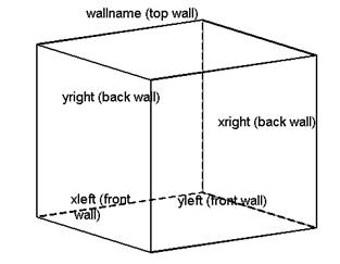
Figure 1: A set of walls relevant for the example input command given above.

Introduction of a membrane boundary condition in LAMMPS

Background

In many physical tests carried out in commercial and research soil mechanics laboratories the samples are confined by membranes that can flex and deform as the sample is compressed vertically. This extra degree-of-freedom in the out-of-plane direction is not possible with the rigid-wall boundaries described above, which overly constrain the displacement field inside a sample. For example a number of very important experimentally observed phenomena (e.g. shear banding) cannot be observed in simulations that use rigid boundaries, leading to inaccurate predictions for the shear properties of granular materials. To allow for the more accurate replication of laboratory test conditions, it was necessary to implement an analogue to a membrane boundary for use with Granular LAMMPS.

Simulations of samples confined by membranes are not often performed as there is no open-source or commercial code available that contains the numerical algorithms required. Furthermore, the routines that implement this are computationally expensive and so in order to run a representative three-dimensional simulation with a sufficiently high number of grains the only solution can be running in an HPC environment. For the above reasons the implementation of a membrane in Granular LAMMPS was assessed as a high priority.

Description of the scheme chosen

A number of schemes have been proposed in the literature as analogues to a membrane as summarised in Cheung and O’Sullivan (2008). They all rely on the calculation of an equivalent weight or area for particles that are within a distance from the edge of the sample, which is then used to calculate external forces applied to the boundary particles - typically the force is the product of this area and a specified pressure. A scheme that implements a numerical membrane can therefore be separated conceptually in three main parts

A. Selection of boundary particles

B. Calculation of an equivalent area for each boundary particle

C. Application of the membrane forces

Initially membrane algorithms were developed for two-dimensional DEM simulations. In this case the solution is less complicated than in the three-dimensional case as the identification of boundary particles is straight-forward. Thomas and Bray (1999) and Cheung and O’Sullivan (2008) used the lengths of the line segments that connect the boundary particles in order to calculate membrane forces by multiplying these by the membrane pressure value. Kuhn (1995), O’Sullivan (2002) and Cheung and O’Sullivan (2008) all extended this concept to three-dimensional simulations by projecting the outermost particle centroids onto planar or cylindrical surfaces. The weight (or area) associated with each particle is then found through the calculation of a two-dimensional Voronoi graph for the points projected on the plane. The additional membrane force is finally set to the membrane pressure value times the area for each boundary particle.

Even though the above represents some aspects of a membrane it has the disadvantage of only applying membrane forces that are perpendicular to the projection plane. A modified algorithm is proposed here so as to relax this condition. The new membrane implementation is thought to be more applicable to cases where the membrane flexes or bulges out of plane, and where the forces would deviate significantly from a direction perpendicular to the membrane projection plane.

In the scheme chosen for this work the starting point for both parts A and B is the calculation of a weighted Voronoi graph (also called Laguerre or radical Voronoi graph – see Okabe et al, 2000) for the system of grains. The entire membrane calculation is implemented as the self-contained class FixMembraneGran, itself derived from the LAMMPS Fix base class. The forces on particles are incremented by the membrane forces through the function post_force() which is executed after the application of the inter-grain contact law for computation of the force on particles due to the contact springs (i.e. after the Pair::compute()command). A more detailed description of the implementation follows.

Voro++, a software library for carrying out three-dimensional computations of Voronoi tessellations

The implementation relies on the use of a Voronoi scheme for the calculation of membrane forces. As in DEM simulations particles often have different sizes (radii) the calculation of a Voronoi graph weighted by radius is most appropriate. Such graphs have been used for DEM before (e.g. Chareyre et al, 2012, Rycroft et al, 2009) but to the author’s knowledge it is the first time that these have been used as part of a membrane calculation. It was therefore necessary to identify a C++ library that included this calculation. Two possible candidates were identified (CGAL and Voro++). Voro++ (http://math.lbl.gov/voro++/), written and maintained by Dr Chris Rycroft of UC Berkeley was chosen as it seemed easier to link into LAMMPS. Furthermore the Voro++ library carries out cell-based calculations, computing the Voronoi cell for each particle individually and so fits in very well with the Granular LAMMPS parallelisation scheme which relies on spatial partitioning of the simulation volume.

At the start of the project Voro++ was not linked to LAMMPS. However, a discussion in the LAMMPS user forum initiated by the author led to the release by the LAMMPS developers of a VORONOI package, which contained extra code that computes a regular Voronoi calculation for a group of particles (through the class ComputeVoronoiAtom). A new class (FixMembraneGran) was added by the author to this package to implement the membrane for granular samples, and a new class to compute the weighted Voronoi (or Laguerre) calculation for a group of grains (the new class ComputeLaguerreAtom). It should be noted that the VORONOI package can be optionally selected by the user to form part of his/her LAMMPS build, if any of the Voronoi or membrane features are required.

Details of the implementation of the new FixMembraneGran class

As a number of operations had to be performed on a weighted Voronoi graph it was not possible to do the graph calculation elsewhere as part of a LAMMPS compute class and then simply communicate the areas required to the class implementing the membrane. Instead all the calculations were included in a new LAMMPS class (FixMembraneGran). The new class contains a number of member functions for initialisation, book-keeping and integration with LAMMPS. The majority of the new code was added to member function post_force(), which gets called once every timestep. It should be noted that should future users wish to speed up their simulations this function could be split into two parts, one that updates the Voronoi graph used for the membrane forces calculation, and one which calculates and adds the extra membrane forces. The update of the membrane forces might then be called less frequently. The function post_force()does the following:

- Initiates two Voro++ container_poly type classes which are used to perform the weighted Voronoi calculations. The coordinates and radii of grains that belong to each processor are then used as inputs to these container classes. The six edges for these containers (required by Voro++ - see the Voro++ documentation) are set by the user through the input script. It should be noted that the code might be made more efficient in the future by only adding grains within a distance from the expected sample edges to these containers.

- Loops through the weighted Voronoi cells in the first Voronoi calculation. For each cell it loops through its set of neighbour cells and checks whether a neighbour with a negative id exists. Note that a negative neighbour id number in Voro++ identifies a cell that would extend to infinity. This step therefore identifies the boundary particles for the sample.

- For each of the cells that extend to infinity it adds the coordinates of an imaginary particle to the container used to calculate the second weighted Voronoi graph. This imaginary particle is added at a distance twice the radius of the boundary particle in the direction towards which infinity was detected. The effect of this is to condition the new truncated boundary cell to pass through a point on the surface of the boundary particle and to have a face parallel to the membrane surface.

- Identifies the faces between the particles in the simulation and the imaginary particles. The areas (n_area ) and their contact normals are used for the force calculation.

- The force to be added to the boundary grains (F_extra) is calculated as

(3)

where p_membrane is the membrane pressure. It should be noted that as n_area is no longer perpendicular to the membrane surface the extra membrane force on the particles is no longer constrained in any specific direction. However the per-particle membrane force is broadly perpendicular to the imaginary membrane surface. All boundary areas are included in the calculation and at the force on a grain is incremented as the calculation progresses.

Testing of the membrane code

The new membrane code was tested on the user’s local machine on a sample of 1600 grains confined by rigid walls on all six sides. After the sample was equilibrated the rigid walls were replaced by membranes on all six sides, with membrane pressures equal to the ones previously applied by the rigid walls. A number of LAMMPS cycles were run and the sample was seen to maintain the stress it was at. A plot of the Voronoi faces that make up the surface of the membrane is shown in Figure 2. Faces with normals parallel to the membrane surface are plotted in red. It can be observed that this new membrane algorithm successfully captures the detail of the sample along its edges and follows accurately the boundary surface of the sample. Simulations using this new membrane boundary condition will now be run for comparison with simulations run with rigid walls. The addition of this new boundary condition allows for the exciting prospect of investigating the formation of shear bands and the observation of the failure mechanism of a laboratory sample of sand, replicated with an accuracy not previously possible in DEM simulations. As a consequence the peak load a given granular sample can sustain will be more accurately predicted too.

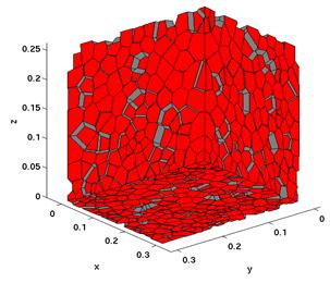
Figure 2: A plot of the membrane faces for a granular sample of 1600 particles.

Compilation of Voro++ on HECToR and inclusion of the VORONOI package in LAMMPS

Both Voro++ and LAMMPS were compiled on HECToR using the GNU compiler. The following command needs to be executed as a first step for both compilations

module swap PrgEnv-cray PrgEnv-gnu

In order to compile the Voro++ libraries (from the source code obtained from http://math.lbl.gov/voro++/download/ ) the following steps had to be performed

- modification of the config.mk file that comes with Voro++: CXX=CC was set (instead of g++) and PREFIX=/home/e***/e***/username/vorodirectory (a directory where the user has write access)

- execution of the command make in the voro++ directory

- followed by make install

In order to compile LAMMPS with the optional VORONOI package the following had to be performed

- the file Makefile.lammps in folder src/VORONOI/ had to be modified by setting voronoi_SYSINC and voronoi_SYSPATH as follows

voronoi_SYSINC = -I/home/e***/e***/username/vorodirectory/include/voro++

voronoi_SYSPATH = -L/home/e***/e***/username/vorodirectory/lib

- execution of the command make yes-voronoi in the LAMMPS src directory to include the VORONOI package code in the LAMMPS build. This should automatically update files Makefile.package.settings and Makefile.package adding voronoi_SYSINC and voronoi_SYSPATH. make yes-granular should also be executed for DEM simulations.

- execution of the command make NAME in the LAMMPS src directory to make LAMMPS using the settings in Makefile.NAME in the src/MAKE directory.

- if a compilation error occurs indicating that the Voro++ library cannot be found it is most likely that the automatic update of the paths above has failed. The user then needs to manually include the voronoi_SYSINC and voronoi_SYSPATH lines in file Makefile.NAME used above, plus the following command

voronoi_SYSLIB = -lvoro++

Use of the membrane boundaries at the input script

The new membrane boundary can be selected through a command of the following format.

fix membranename all membrane/gran ${xleft} ${xright} ${yleft} ${yright} ${zbottom} ${ztop} ${pressurex} ${pressurey} ${pressurez} ${distx} ${disty} ${distz}

A membrane boundary (fix of type membrane/gran) with name membranename is created. Parameters enclosed in ${} signify LAMMPS style variables that specified through a variable equal command at the input script. Numerical values can also be specified for these directly. Values for xleft, xright, yleft, yright, zbottom and ztop are the bottom and top limits in the x, y and z Cartesian axes directions respectively for the container used in the calculation performed by the Voro++ library. These should be set to be roughly coincident to the locations of rigid walls that would form an imaginary container bounding the whole assembly of grains in the sample.

Arguments pressurex, pressurey and pressurez are the membrane pressures for the faces perpendicular to the x, y and z axes respectively. Here a positive value signifies an additional inward force for the sample (i.e. compression is positive). If any of these arguments is specified as NULL there are no extra membrane forces applied to the boundary particles for that particular set of faces. This could be the case when a rigid boundary is selected for this direction, for example. Arguments distx, disty and distz specify distance values necessary for correct calculation of membrane forces when the code is run in parallel. They should be set to values lower than the width of the minimum subdomain in the direction in question (x, y or z) but should be larger than the expected distance of the centroid of a boundary particle from the edges of the Voro++ container. When LAMMPS is executed in parallel a Voronoi calculation is performed at every processor and inclusion of these parameters ensures that membrane forces are only added for grains that are at the edges of the sample, and not at inter-processor boundaries.

Extension of the contact models (pair styles) available in Granular LAMMPS

Background

In LAMMPS the inter-particle interaction is coded inside the Pair classes. A large amount of effort has gone into developing these for Molecular Dynamics simulations. However the Granular LAMMPS package which enables DEM simulations only contained a few basic models. These included a linear and a non-linear elastic contact spring, with each inter-particle interaction law implemented as a separate Pair class. A new non-linear elastic contact spring model was created which was more representative of a Hertz-Mindlin elastic contact most appropriate for DEM simulations of frictional grains. However the main aim of the second Work Package of this project was the addition of an interaction law for bonded particles, making possible simulations of porous rocks and opening up the use of HPC to DEM users in the geological sciences, among others.

Addition of the PairGranShmHistory class

Dr Kevin Hanley and Mr Xin Huang, members of the Imperial College LAMMPS developer team identified that the non-linear elastic interaction law in class PairGranHertzHistory differed from the Hertz-Mindlin interaction (see Mindlin and Deresiewicz, 1953 or Itasca, 2003) commonly used in DEM simulations. The calculation of normal force (i.e. force in the direction of the vector connecting the centres of two contacting particles) was that predicted by Hertzian theory (Johnson, 1985) but the interaction in the plane perpendicular to that (i.e. the shear or tangential interaction) differed. It was therefore thought appropriate to add a new pair class (PairGranShmHistory) that implements a Hertz-Mindlin interaction. It should be noted that addition of a new class instead of modification of the existing one was thought best for backwards compatibility issues.

The new class was implemented as a child of the PairGranHookeHistory class and so shares a number of member functions necessary for Pair classes with it. The computation of inter-particle forces (as redefined in the compute() function) is very similar to the one for other granular classes, a key difference being that the quantity stored in the per-particle shear[] array is now the shear force from the previous timestep and not the extension of the shear spring as in PairGranHookeHistory or PairGranHertzHistory . As mentioned above the normal force in this new interaction model is identical to the one in PairGranHertzHistory::compute() for no contact damping. The shear force equation implemented here however is the following:

(4)

where is the increment in the shear force at the current timestep, G is the grain materials shear modulus, v the Poisson ratio, δ_n the displacement of the normal spring (i.e. the grain overlap), R_A and R_B the radii of the two contacting grains, Δt the timestep value and Δu_shear the rate of extension of the tangential spring. It should be noted that no contact dashpot was implemented in this Pair style as there are other LAMMPS fix classes (e.g. FixViscous) that can be used to damp out oscillations in DEM simulations. Also, to enable use of this new interaction law in DEM simulations with flat boundaries the function shm_history() was added to the class that implements the flat boundaries (FixWallGran). The new pair class was then used for the simulations discussed on page 16, and an example command will be given at the end of this section.

The PairGranHookeHistoryPbond class that implements the new bonding model

A number of bonding models have been proposed for use with DEM simulations (Potyondy and Cundall, 2004, Utili and Nova, 2008, Weatherley, 2009). Of these the model proposed by Potyondy and Cundall is the one most often used. Members of the Imperial College LAMMPS users group have used this model before in a number of simulations (Marketos and Bolton, 2009, Hanley et al, 2010, Cheung and O’Sullivan, 2008) when using other serial codes and so it was thought that addition of this model to Granular LAMMPS was most appropriate.

There were two options for implementing the new bonding model in Granular LAMMPS. This could be done through the use of either a bond style, or a pair style. The bond style offered the advantage of a self-contained scheme for the calculation of the interaction forces between bonded grains. However in LAMMPS such bond styles are only available for Molecular Dynamics simulations. The challenge when adopting LAMMPS bonds for Discrete Element simulations was that in DEM extra per-bond memory needs to be allocated for the bond state information. This memory then needs to be copied across processors when grains move through processor boundaries and dealt with properly when bonds get added or removed from a bond list.

Instead the author chose to implement the bonded model as a Pair class in LAMMPS. This offered the advantage of using the contact list (called a neighbor list in LAMMPS) to store the bond state information. The granular neighbor list logic is well-established in LAMMPS and has been tested and debugged by numerous users over the past years. It therefore provided a safe way of proceeding with the implementation of a bonded model in the limited time available for this project. The following was necessary as part of the new PairGranHookeHistoryPbond class.

- The number of per-contact quantities stored with the granular neighbor list had to be increased. This was done through a modification to the FixShearHistory class so that it takes an extra argument, the number of per-contact quantities to be allocated. The default number of such quantities for granular pair styles in LAMMPS was 3, but the new bonded model required 12 per contact quantities. Entries 0 to 2 of this per contact array were reserved for the three Cartesian components of the extension of the shear spring, similar to what was implemented in the PairGranHookeHistory class. Entry 3 was a number set to 1.0 for bonded contacts or -1.0 for unbonded ones and entry 4 contained the equilibrium distance for the bond normal springs, used to calculate the bond force in the direction of the inter-grain contact normal. Entries 5 to 7 were reserved for the Cartesian components of the shear bond force and 9 to 11 for shear bond moment, while entry 8 contains the bond moment in the direction of the inter-grain contact normal. Conversations with Dr Christoph Kloss (JKU Linz, Austria) when adding to the per-contact quantites list were very useful.

- A compute() function was coded. This implemented the equations as described in Potyondy and Cundall (2004).

- A pbondflag was introduced to indicate whether a bond exists at a specific contact.

- Bond creation was dealt with inside the compute() function. A createflag was used to indicate whether parallel bonds should be installed at all eligible contacts, typically at the start of a simulation. The condition for bond installation was that the overlap between two spheres should be larger than a specific value (d_install). If no d_install value was set by the user the default behaviour was to install bonds at all contacts where there was overlap. A negative value of d_install meant that bonds would be installed to connect non-overlapping contacts while a positive value meant that only contacts with overlaps greater than d_install would be bonded. Bond creation was only allowed in the beginning of a simulation, or after the execution of a pair_modify command.

- Bond breakage was checked for at every timestep. This was done inside the compute() function. The normal and shear bond stress were calculated and if these exceeded a certain normal or shear stress the bond was set to break either in tension, compression, shear or torsion. After bond breakage the inter-particle interaction reverted to that of a contact spring alone.

Verification of the bonded interaction model

Cheung (2010) detailed the results of an investigation of the behaviour of a two-grain bonded system in commercial code PFC3D, which implements the model of Potyondy and Cundall (2004). Two-grain simulations identical to the ones presented in Cheung were performed here with a serial executable of LAMMPS in order to verify the implementation for the bonded model. In these simulations two grains (A and B) of a radius of 0.5m were created just touching each other. The velocity and angular velocity of grain A were set to zero and grain B was moved with both contact springs and a parallel bond installed at the contact. A sketch of the 2-grain initial positions is given in Figure 3. Figures 4, 5 and 6 plot the results for simulations of inter-grain movement in the normal and shear directions and for spin about the contact normal. The relevant figures from Cheung (2010) are also shown for comparison. As the results agree very well the current implementation of the inter-particle bonded interaction is verified.

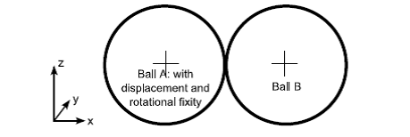
Figure 3: A schematic of the 2-grain arrangement used for the bonding model verification simulations (after Cheung 2010)

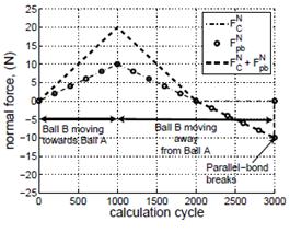
(a) (b)

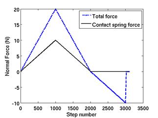
Figure 4: The results for inter-grain movement in the normal direction (creating tension in the bond). Note that after 3000 steps the bond breaks. (a) LAMMPS and (b) Cheung (2010) results using PFC^3D.

(a) (b)

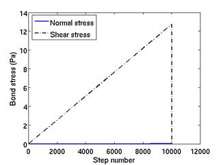
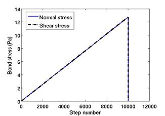
Figure 5: The results for inter-grain movement in the shear direction. Note that after 10000 steps the bond breaks. (a) LAMMPS and (b) Cheung’s (2010) results using PFC^3D.

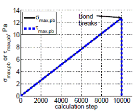
(a) (b)

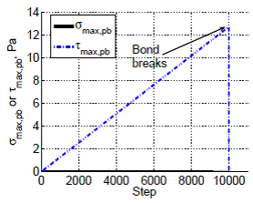
Figure 6: The results for the case when one grain spins relative to the other. Note that after 10000 steps the bond breaks. (a) LAMMPS and (b) Cheung’s (2010) results using PFC^3D.

Use of the new inter-grain interaction models at the input script

The modified Hertzian spring can be selected through the following command

pair_style gran/shm/history ${G} ${Poisson} ${mu}

Here the last three arguments are the shear modulus, Poisson ratio and frictional coefficient for grains respectively. These can be enclosed in ${} and specified as LAMMPS style variables through a variable equal command preceding the pair_style command, or specified with their numerical values directly. The above command needs to be followed by

pair_coeff * *

for compatibility with other LAMMPS pair commands. In cases where a granular wall is needed with the new modified Hertzian model this should be specified through a command of the type:

fix wallname all wall/gran ${G} ${Poisson} 0.0 0.0 ${xmu} 0 zplane NULL 0.1

where the format of the wall command with all its optional arguments is followed and the only wall parameters needed are the shear modulus, the Poisson ratio and the frictional coefficient describing the behaviour of the ball-wall contact.

The new bond model can be specified through the command

pair_style gran/hooke/history/pbond ${kn} ${kt} ${xmu} ${kbn} ${kbt} ${nstrength} ${sstrength} ${bradmul} ${d_install}

where kn and kt are the linear contact spring normal and tangential stiffnesses and xmu is the frictional coefficient for the contact. kbn and kbt are the spring bond stiffness densities, nstrength and sstrength the normal and shear strength of the bond that controls bond breakage. bradmul is the ratio of the minimum radius of the two grain assembly that is used as a radius for the bond disc and d_install is the overlap above which bonds should be installed. Note that a negative value for this means that bonds will be installed between non-contacting grains too. Again this pair command needs to be followed by pair_coeff * *.

A large-scale simulation that makes use of the new features implemented

A large-scale simulation was performed in an HPC environment so as to illustrate the potential of the use of granular LAMMPS. 1.95 million grains were rained under gravity and were equilibrated inside a container similar to the one shown in Figure 1. The grain properties (e.g. grain size, density, stiffness) were representative of a sample of fine glass beads used by experimentalists in Bristol University in an ongoing EPSRC funded research project (EP/G064180/1), and the sample container had the same dimensions as the laboratory container. After raining of the particles the top was flattened by removing approximately 500,000 grains so that the sample used for the subsequent simulations contained 1,428,532 grains. The timestep chosen for this simulation was chosen according to published guidelines (see Itasca, 2003) and a stressing simulation was set up, with a stress rate of 200kPa/sec for all six sides of the sample container, by using the commands described above.

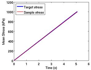
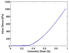
The mean stress versus time and mean stress versus volumetric strain for the simulation are given in Figures 7a and 7b below. In Figure 7a it is clear that the sample stress indeed followed the target stress for the stress-controlled moving wall. Figure 8 shows the results for a simulation where the gain parameter was incorrectly chosen to be too low; here a system instability can be observed as the wall stress oscillates above and below the target stress. An appropriate value for the gain parameter for the stress-controller was found by trial and error here; identification of this is the topic of further work, but it should be a function of the sample stiffness and stress rate. This is due to the fact that its value must depend on how fast the target stress changes in a given timestep, and on how much the boundary velocity affects the boundary force (i.e. what is the value of the tangent to force-displacement curve for a boundary)

(a) (b)

Figure 7: Stress-controlled compression of a sample of 1.43million grains (a) A plot of stress versus time (b) Mean stress versus volumetric strain.

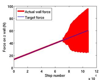
Figure 8: Stress-controlled compression of a sample of 1.43million grains: Sample instability for incorrect choice of the stress-controller gain parameter.

The sample, which was stressed at 100kPa was then used for a simulation of wave propagation from a point source, analogous to a bender element laboratory test. This test is commonly used in the laboratory for determination of the shear stiffness of a soil sample but the signals produced are poorly understood. As part of the above-mentioned EPSRC-funded research project (EP/G064180/1), co-workers at Imperial have simulated a bender element test in smaller DEM simulations (see O’Donovan et al, 2012). Simulations that have used HECToR have led to wave propagation virtual experiments in larger samples (see Fig. 9 for a received signal for one such simulation). As briefly discussed above the use of HPC has allowed for the direct replication of a laboratory test conducted by collaborators at Bristol University on a material with much smaller grains. This is very important as it has allowed for an increase in the number of full wavelengths that can be contained within the sample and an increase in the wavelength to mean grain size ratio, both of which affect profoundly the wave propagation patterns observed. With this larger simulation it was therefore possible to investigate more representative values for these parameters and identify their exact effect of the signals received. Wave velocities, differences in the shapes of the propagated signals and the exact wave propagation patterns within the samples will all now be analysed with the aid of the data collected on the larger samples.

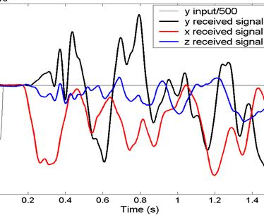
Figure 9: The input and received signals for a point-wave excitation simulation on a sample of 1.45million grains that was stressed at 100kPa on HECToR.

Outcome of the work and future prospects

The simulation illustrated above represents a milestone for both the author and the research area. It contains 30 times more particles than anything attempted before by the author, while total simulation times, including sample preparation were not in excess of six weeks. Sample preparation was performed on cx1, the HPC cluster at Imperial College London, on 72 cores using an infiniband inter-connect and took approximately a month. The subsequent stressing was performed on HECToR using 8 fully populated nodes (256 cores) and took approximately 48 cpu hours to reach a stress of 1MPa representing a total simulation time of 5 seconds, i.e. a total of more than 20million timesteps. We have been monitoring the size of simulations used in DEM simulations for geomechancis applications (e.g. O’Sullivan, 2011) and we know of no other study where analysts have simulated in excess of 1 million particles and compressed the particle assembly in a controlled manner. This is therefore a significant development for the research field.

At the start of the author’s involvement granular LAMMPS we were not aware of any UK academic running DEM simulations in an HPC environment. At the moment the Imperial College DEM user group has four members, all of which are using HPC for their DEM simulations and another member who is investigating the use of granular LAMMPS and is considering adopting it over a commercial serial code he is using. Simulations are currently being run on a number of very diverse topics. These include simulations of wave propagation through sand, of tunnelling through soil, of internal erosion through dam structures, of cyclic loading of sand, and of liquefaction of sand. We are aware of the use of granular LAMMPS on research projects directed by Dr Xia Li of Nottingham University and Dr Jin Sun of Edinburgh University, both of which will benefit from the developments resulting from the project described here.

The author and co-workers are in the process of producing a publication in an international refereed journal which will contain a description of simulations conducted using the new features added to LAMMPS here. This will attract attention to the use of HPC for DEM simulations and will act as a tangible proof of the potential of the combined use of granular LAMMPS and HECToR for high-impact science. It is thought that this will attract a number of new users to HECToR; the author has already demonstrated the use of HECToR to colleagues at Napier University for example. Furthermore, the developments detailed here will allow more DEM users to move away from commercial codes and free up EPSRC funds that were otherwise spent on software licences. It should be finally noted that all developments detailed here are already part of the Imperial College LAMMPS version that is shared between researchers locally. The author has contacted Dr Steve Plimpton (the main LAMMPS developer) with the intent of adding the new LAMMPS classes to the main distribution. Efforts are also underway to add these to the LIGGGHTS codebase (a software effort also based on granular LAMMPS) through discussions with Dr Christoph Kloss, one of its main developers. In the meantime the new features will be publicised through replies to active discussion topics in the online LAMMPS user forum.

Acknowledgements:

This project was funded under the HECToR Distributed Computational Science and Engineering (CSE) Service operated by NAG Ltd. HECToR – A Research Councils UK High End Computing Service - is the UK's national supercomputing service, managed by EPSRC on behalf of the participating Research Councils. Its mission is to support capability science and engineering in UK academia. The HECToR supercomputers are managed by UoE HPCx Ltd and the CSE Support Service is provided by NAG Ltd. http://www.hector.ac.uk

The author would like to thank Dr Catherine O’Sullivan for her support and encouragement throughout this project. Discussions on the implementation with her and with Dr Kevin Hanley also of Imperial College London are gratefully acknowledged. Dr Steve Plimpton and Dr Paul Crozier (Sandia National Labs), Dr Christoph Kloss (Johannes Kepler University, Linz) and Daniel Schwen also deserve a mention for their invaluable discussions and help. The author would also like to thank Dr Phil Ridley (Numerical Algorithms Group Ltd) for his support.

References

Chareyre B, Cortis A, Catalano E & Barthélemy E (2012). Pore-Scale Modeling of Viscous Flow and Induced Forces in Dense Sphere Packings. Transport in Porous Media, Vol. 92, No. 2, pp 473-493.

Cheung G & O'Sullivan C (2008). Effective simulation of flexible lateral boundaries in two- and three-dimensional DEM simulations, Particuology, Vol. 6, pp. 483-500.

Cheung, G. (2010). Micromechanics of sand production in oil wells. Ph.D. thesis, Imperial College London.

Cundall, P. (2001).A discontinuous future for numerical modelling in geomechanics? Geotechnical Engineering Proceedings of the Institution of Civil Engineers 149 (1), 41–47.

Cundall, P. and O. Strack (1979a).A discrete numerical model for granular assemblies.Geotechnique 29 (1), 47–65.

Cui L, O’Sullivan C & O’Neill S (2007). An analysis of the triaxial apparatus using a mixed boundary three-dimensional discrete element model. Geotechnique, Vol. 57, No. 10, pp. 831-844.

Hanley (2013) personal communication.

Hanley, K., O’Sullivan, C., Byrne, E. P. , Cronin, K. (2012) Discrete element modelling of individual agglomerates of infant formula. Particuology, 10(5), pp 523-531.

Itasca Consulting Group Inc. (2003). PFC3D: Particle Flow Code in 3 Dimensions, Version 3.0, Minneapolis, USA.

Johnson, K. (1985). Contact Mechanics. Cambridge University Press.

Kuhn MR (1995). A flexible boundary for three-dimensional DEM particle assemblies. Engineering Computations, Vol, 12(2), pp. 175-183.

Marketos G & Bolton MD (2009). Compaction bands simulated in Discrete Element Models, Journal of Structural Geology, Vol. 31, pp. 479-490.

Marketos G & Bolton MD (2010). Flat boundaries and their effect on sand testing, International Journal for Numerical and Analytical Methods in Geomechanics, Vol. 34, pp. 821-837.

Mindlin RD & Deresiewicz H (1953). Elastic spheres in contact under varying oblique forces. ASME Journal of Applied Mechanics Vol. 20, pp. 327-344.

O'Donovan J, O'Sullivan C & Marketos G (2012). Two-dimensional discrete element modelling of bender element tests on an idealised granular material. Granular Matter, Vol. 14, pp. 733-747.

O’Sullivan, C (2002). The application of discrete element modelling to finite deformation problems in geomechanics. Doctoral Dissertation, University of California, Berkeley.

O’Sullivan C (2011). Particulate Discrete Element Modelling: A Geomechanics Perspective. Taylor and Francis, London.

Okabe A, Boots B, Sugihara K & Chiu SN (2000) Spatial tessellations: concepts and applications of Voronoi diagrams. 2^nd Edition, Wiley.

Potyondy, DO and PA Cundall (2004). A bonded-particle model for rock. International Journal of Rock Mechanics and Mining Sciences, Vol. 41(8), pp. 1329-1364.

Rycroft CH (2009). Voro++: A three-dimensional Voronoi cell library in C++, Chaos Vol.19, 041111

Shen C-K (2012) PhD Thesis, Imperial College London

Thomas P & Bray J (1999). Capturing nonspherical shape of granular media with disk clusters. Journal of Geotechnical and Geoenvironmental Engineering, Vol. 125(3), pp.169-178.

Utili, S. and R. Nova (2008). DEM analysis of bonded granular geomaterials. International Journal for Numerical and Analytical Methods in Geomechanics 32 (17), 1997–2031.

Weatherley, D. (2009). Esys-particle v2.0 users guide. Technical report, Earth Systems Science Computational Centre, University of Queensland.