For over half a century it has been a goal to produce energy inexpensively from nuclear fusion. Confining the fusion plasma inside magnetic fields is presently the most promising approach to achieve this goal. To achieve this, further advances in both experiment and theory are required. Modelling fusion plasmas using high performance computing is a key tool to further our theoretical understanding of the problem. Due to the large range of spatial and temporal scales involved, applications typically model only specific aspects of the fusion plasma. This project worked on the application GS2, which uses the gyrokinetic approach to investigate micro turbulence within the fusion plasma.

The flux-tube gyrokinetic code GS2 is an initial value code that solves the gyrokinetic equations for the perturbed distribution functions together with Maxwell’s equations for the turbulent electric and magnetic fields. GS2 is a mature open source code written in Fortran90. It was originally developed in the US by Dorland, Kotschenreuther and Liu. It is parallelised using MPI and offers a number of different parallelisation schemes, which can be switched at runtime. The source files contain over 65000 lines in 60 files.

By integrating over the Larmor motion, the six dimensional phase space is reduced to 5 dimensions. As a consequence the data structures in GS2 are five dimensional. The advance in time is calculated, with the two perpendiculars to the field position space coordinates in Fourier space (aka. k-space). The non-linear terms are, however, best calculated in position space. For the required fast Fourier transformations (FFT) GS2 deploys version 2 of FFTW library. In 2003 version 2 of FFTW got replaced by version 3. In contrast to version 2, FFTW version 3 is capable of utilising the SSE instructions offered by modern processors, promising to be a better performing FFT library. When releasing FFTW version 3, FFTW version 2 became legacy code, which is no longer actively supported by its developers. Upgrading GS2 from FFTW2 to FFTW3 is the key aim of this HECToR dCSE project. Since the interfaces to FFTW2 and FFTW3 are incompatible, upgrading GS2 to FFTW3 involves significant re-engineering.

This document reports the work done to upgrade the FFTs in GS2. Section 2 gives a brief comparison between the FFTW2 and the FFTW3. An analysis of the existing GS2 code is described in the Section 3. Section 4 shows the performance study of the GS2 accelerated transform implementation and the details of its re-engineering work are explained in the Section 5. Section 6 describes the investigation on the non-accelerated transform implementation and the related Totalview results are listed in the appendix for details, after the report conclusions in Section 7.

2. FFTW version 2 and FFTW version 3

The FFTW library is a widely deployed library to calculate fast Fourier transformations in scientific codes. The source is available for download from the FFTW website (www.fftw.org). On the HECToR system FFTW version 2 and version 3 are provided by Cray as part of the system software. As noted before the interfaces of these versions are incompatible. In the next sub-section we will outline the key issue.

2.1 FFTW2 and FFTW3 interface

In this subsection we will shortly outline the key differences between the user interfaces of FFTW2 and FFTW3. For a more in-depth discussion we refer to the documentation available from the FFTW website.

The key difference between the two libraries is that in FFTW3, the input and output arrays need to be known at the time of plan creation, while for FFTW2 they are not required at this stage. Knowing the input and output arrays, FFTW3 can examine the alignment properties of these arrays to deploy the SSE instructions and hopefully deliver better performance over its predecessor. In the latest releases of FFTW3, plans can be reused for other arrays than the ones used at plan creation, provided that these arrays have the same alignment properties as the original ones. However this is hard to control in a portable way in Fortran.

GS2 utilises the advanced interface of FFTW which allows for several FFTs to be calculated in a single call. In FFTW3 this requires a proper description of the data layout, such as the stride between individual elements and the distance between transformations, at the time of plan creation. Also the number of FFTs that requires calculating needs to be known at plan creation. GS2 has a separate module to create the plans for the FFT. Since FFTW2 does not require this information for the plan creation, in the original GS2 code the additional information required for FFTW3 is not available to the module creating the plans. Re-engineering of the application is required to make the information available.

A further complication is, if there are arrays that need transforming, which have the same size for the FFT, but differ with respect to their data layout or the number of FFTs that need calculating, they can in FFTW2 use the same plan. In FFTW3, different plans are needed, since the data layout and the number of FFTs needs to be specified at the plan creation stage.

2.2 FFTW3 performance on HECToR

At the application stage of the proposal, we performed a simple benchmark comparing the performance of FFTW2 and FFTW3 for a simple FFT using one dimensional input and output arrays of complex numbers. The benchmark repeatedly calculates the same FFT to obtain stable timings. The results are shown in Figure 1.

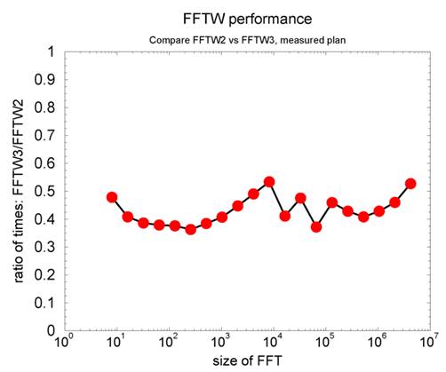
Figure 1 Performance comparison for a simple benchmark

The results suggest a performance improvement of about a factor of 2, even for input data exceeding the size of the L3 cache of 2 MB shared between the four cores. Since GS2 can spend substantial amounts of time in the FFT library, it was hoped at the proposal stage, that an upgrade from FFTW2 to FFTW3 would give similar performance improvements for GS2.

FFTW2 is now a legacy library, which is not developed an updated any more. Upgrading GS2 to use FFTW3 will move the code to a contemporary library which is still supported by its authors.

3. Analysis of the existing code

As described, in the case of GS2 the upgrade requires re-engineering of the code. To facilitate changes to the code, a deep understanding of the existing code is required. This section gives an overview of the code analysis carried out during this project.

3.1 Routines which access the fft type variables

Most FFT libraries (including FFTW) require a two stage process to calculate an FFT. This way, many expensive calculations, such as the evaluation of trigonometric functions, are called once and the result is then stored for future use. This first step is typically called “plan creation”. Assuming the same FFT is executed many times this is typically more efficient. To pass information between the plan creation step and to the actual calculation of the FFT, FFTW uses a handle, which in Fortran gets declared as an 8-byte integer.

One can learn a lot about the existing code, by investigating which parts access these integer variables commonly called “plan”. In GS2 these variables are stored in a type-definition called fft_type. These are defined as:

type :: fft_type

integer :: n, is, type

integer (kind_id) :: plan

real :: scale

end type fft_type

and contain a member “plan”. The file gs2_transforms.fpp has seven variables of the above described derived type type :: fft_type. Their names are:

xf_fft, xb_fft, yf_fft, yb_fft, zf_fft, xf3d_cr, xf3d_rc

The plans associated with xf_fft, xb_fft, yf_fft, yb_fft, zf_fft are not destroyed during execution of the program. The plans associated with xf3d_cr, xf3d_r will be deleted by init_3d, if they are associated with different sized transformations than required.

Figures 2 – 5 detail the usage of xf_fft, yf_fft, zf_fft, xf3d_cr, xf3d_rc. The variables xb_fft and yb_fft are associated with the backward transformations matching onto xf_fft and yf_fft and are used in a similar fashion. For the understanding of Figures 2 and 3 it is helpful to know how the parallelisation effects the transformations.

For smaller numbers of processors, both the x and y direction are local to the processor. In this case GS2 performs what it calls an “accelerated” transformation. A single plan is created to perform a set of 2D FFTs in a single call and xf_fft and xb_fft are never accessed throughout the entire program execution. In this case the actual FFTs are calculated by calling transform_5d_accel (via the interface transform2).

For large number of processors, the x and y directions get distributed. In this case two plans for the forward transformation (associated with xf_fft and yf_fft) and two plans for the backward transformation (associated with xb_fft and yb_fft) get created. The actual transformations are calculated by doing each direction x and y separately by first calling transform_x5d and then transform_y5d. In this case, transform2_5d_accel is not accessed during program execution.

use_of_yf_fft

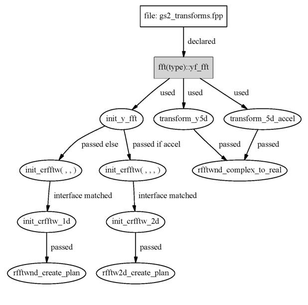
Figure 2 Access to yf_fft

use_of_xf_fft

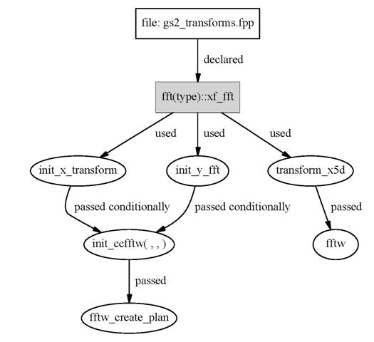
Figure 3 Access to xf_fft

use_of_zf_fft

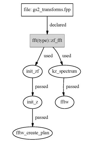
Figure 4 Access to zf_fft

use_of_xf3d_cr_rotated

Figure 5 Access to xf3d_rc and xf3d_cr

3.2 Call structure of fft interfaces

GS2 uses Fortran interfaces to make the code for initialising and accessing the transformations more legible. To better understand how these interfaces work, the project documents which routines are called when the interface gets accessed. A graphical representation of this analysis is given in Figures 6 and 7.

Figure 6 shows the call tree for the interfaces transform2, transform_x and transform_y. The code contains similar interfaces inverse2, inverse_x and inverse_y, which are not documented here, since they are the inverse of the above. They are easy to understand once the transform interfaces are understood.

The interface transform2 matches onto five different routines. The chosen routine depends on the number and dimensionality of the arguments:

transform2_5d: this is chosen if transform2 is called with 2 arguments

transform2_5d_accel: this is chosen if transform2 is called with 3 arguments

transform2_4d: this is chosen if transform2 is called with 4 arguments and the first argument is a 4 dimensional array

transform2_3d: this is chosen if transform2 is called with 4 arguments and the first argument is a 3 dimensional array

transform2_2d: this is chosen if transform2 is called with 4 arguments and the first argument is a 2 dimensional array

We like to note that there is no inverse to transform2_4d. The call structure in Figure 6 also shows that the routines transform2_4d, transform2_3d and transform2_2d call their respective initialisation routines. These routines, not shown in the figure, create the required plans and there is no public interface to allow plan creation in any other way. This shows that the present routines are not set up to achieve the highest performance, but for functionality. Since these are not called during critical parts of the benchmarks used so far in the project, at present we do not believe this presents a performance issue.

Figure 7 shows the call structure for the public subroutines used to initialise the transformations. Of particular interest is the public subroutine init_x_transform. In the present version of the code this does not get called at all. As visible in the graph, if plans for the x transforms are required, these get created by init_transforms. This is for large processor counts, if the variable accel is set to false, marked as “non-accel” in the figure.

gs2_transform_call_graph_rotate

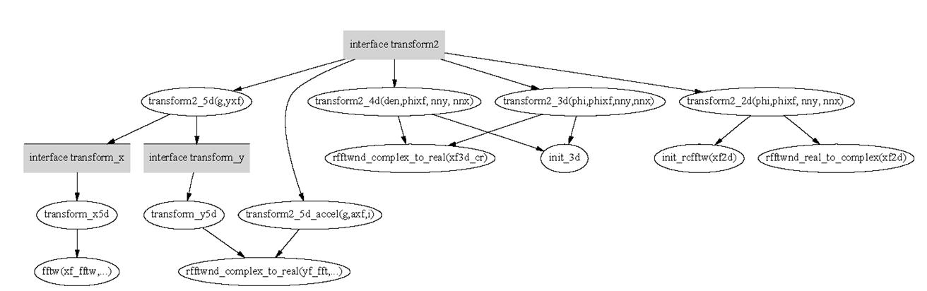
Figure 6 Call structure of the interfaces associated with the exectution of the FFT transformation

init_transform_call_graph

Figure 7 Call structure of the public subroutines required for the initialisation and plan creation for the FFTs

3.3 Callers of the transformations

Figures 8 and 9 show the routines in GS2 that access the interfaces transform2 and kz_spectrum. For the interface transform2, we show the name of the actual routine called instead of just the interface name. The figure shows that the routines transform2_3d, transform2_4d, inverse2_2d and inverse2_3d are only used in either the initialisation or the diagnostic part, which are not critical to performance.

references_to_fft_stuff_bottom

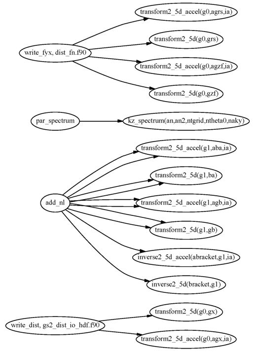
Figure 8 Routines accessing the interface transform2 (part 1)

references_to_fft_stuff_top

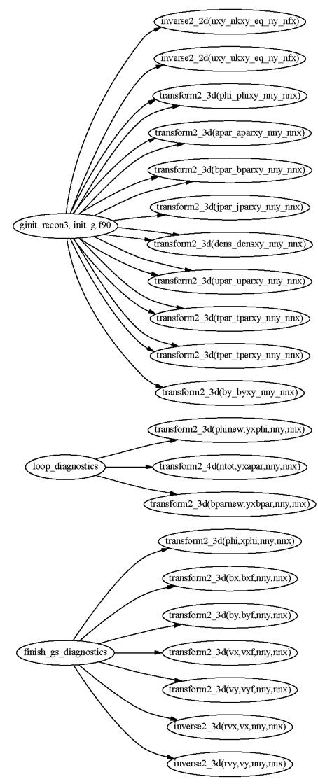
Figure 9 Routines accessing the interface transform2 (part 2)

Figure 10 shows routines that access transform_x and transform_y. The interfaces transform_x and transform_y are presently only accessed from transform2_5d.

references_to_xy_fft_stuff

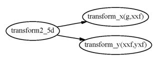
Figure 10 Routines accessing the interface transform_x and transform_y

The last Figure of this section, Figure 11 shows access to the initialisation routines.

references_to_init_fft

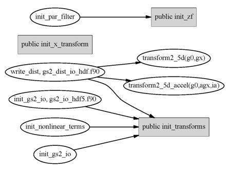
Figure 11 Routines calling the initialisation routines

3.4 Input data of Complex-to-Real transformations

When using the advanced interface of FFTW, complex-to-real transformations will destroy their input data: see the FFTW user guide for details. We confirmed that the routines transform_y5d, transform2_5d_accel, transform2_4d, transform2_3d and transform2_2d, which perform complex-to-real transformations, copy the data into a work buffer, which in turn is passed as an input array to FFTW. While this has disadvantages from a performance point of view, it prevents the destruction of data that is still needed.

4. Benchmark Studies

The project performed two benchmark style studies to guide the coding, and these studies were performed outside GS2 using a test-harness suite. The first checked on the importance of controlling the alignment of input and output data. The other study was to investigate the best strategy for deploying FFTW3 within transform2_5d_accel.

4.1 Importance of 16-byte alignment

A question that arose during the dCSE meeting in September 2009 in Oxford was, whether the alignment was still an issue or whether modern compilers and processors could deal with any alignment, when using SSE. GS2’s data structures use 8-byte real (aka. double precision) variables. For complex variables this translates into 16-byte numbers. For a double precision code, the processor can access two words from the cache line simultaneously, but needs different instructions depending on the location of the words on the cache line with respect to the 16-byte boundary.

We conducted a simple test, which sets up a complex-to-complex transformation using dfftw_plan_dft_1d and a real-to-complex transformation using dfftw_plan_dft_r2c_1d. The FFTW3 commands dfftw_execute_dft and dfftw_execute_dft_r2c then allow deploying these plans to transform arrays different from the ones used at for the plan creation. By handing e.g. a(0) of an array a declared as 8-byte real numbers to FFTW3 for the plan creation and then handing e.g. a(1) as input data to dfftw_execute_dft_r2c for the execution, one can test how the code reacts when differently aligned data are used for plan creation and execution.

We noticed that this code crashes in a non-deterministic way. On repeated runs this code core dumps in different places. The reason for this non-deterministic behaviour might be operational noise during plan creation. In FFTW it is not guaranteed that repeated runs use the same plan.

We did not notice any problems, for the complex-to-complex transformation when using shifted indices. This is expected since these variables occupy 16-byte each and are naturally aligned by most compilers.

The conclusion of this test is, that when modifying GS2, we have to control the alignment of real input or output data, when plans are used for arrays different from the ones used at plan creation.

4.2 Performance study of 2D FFT for transform2_5d_accel

When having the x and y (or their respective Fourier space coordinates) processor local, the initial version of GS2 issues calls to rfftwnd_f77_complex_to_real and rfftwnd_f77_real_to_complex to calculate a number of 2D FFTs within a single call.

We assumed fairly typical array dimensions from GS2 simulations, and set up the code so that each call calculates 62 FFTs of dimension 96 ´ 96. The input data are laid out in the program such that the data points belonging to the same FFT, are separated by 61 data point belonging to other FFTs.

The obvious question is, whether it is more advantageous to rearrange (transpose) the data, such that data points belonging to the same FFT are subsequent, followed by the data required for the next FFT and so on. Obviously, the strided copy required for the transposition of the data will also be expensive. We conducted a small simple test to determine what is effective on the present HECToR.

To avoid alignment issues when using SSE instructions, one can declare input and output work arrays for all FFTs. These work arrays are supplied to the planning routines. When conducting the actual FFTs, the input data, as supplied by the code, need to be copied into the input work array that was used for plan creation. Once the FFT has been completed, results must be copied from the output work array into the place where the code requires this data. The aim of this study is to examine whether the additional cost of a strided copy over a straight copy can be recouped by the actual FFT becoming faster with the improved data layout.

An alternative is to use FFTW3 without any SSE, which can be accomplished by adding FFTW_UNALIGNED to the flags at the planning stage. This way, the plan is safe to be reused on any array, irrespective of its alignment, and if one keeps the original strided data layout no additional copy is required.

The Benchmark

For the benchmark, we compared 6 strategies in the code. In 1-5 we copied data into the FFT input array, performed the FFT, and copied the output into a result array.

1. Simple copy that preserves the original data layout. Using the PGI 10 compiler, explicit loops tended to give better performance than using Fortran array syntax.

2. Transpose the data and copy into a single array with more efficient “normal” order: ie first all the data of the first FFT followed by the data for the second FFT and so on. The 62 FFTs are performed in a single call.

3. Copy into a smaller input array, which holds the data for a single FFT. This also involves a strided copy of the data. This technique might be more cache friendly.

4. Copy into a small input array, which can hold the data for two FFTs. The hope was, that this would benefit from better cache reuse, being more cache efficient with respect to the copy.

5. Abandon SSE instructions by using the FFTW3 planning flag FFTW_UNALIGNED, which should lead to a performance penalty, at least when using data which can be cached on the highest cache levels. The advantage of using this flag is that it resolves alignment issues, and the plans can be used in a similar fashion to FFTW2: i.e. any array with the right size and data layout can be transformed using fftw_executed_dft_r2c. It is interesting to assess how much of a penalty this involves for the GS2 data structures. Copies preserved the original data layout.

6. No copies. Having tested the FFTW_UNALIGNED, it is also interesting to test, how the performance changes if FFTW works directly on the data without copies into input and output buffers. For GS2 this is not fully applicable due to the anti-aliasing. There has to be an output buffer in case of a real-to-complex transformation. Without a copy, the inverse 2D complex-to-real FFT cannot preserve the input data (as is required in GS2). Hence at least one data copy is needed in GS2.

This code was compiled using version 10.0 of the PGI compiler and executed on the HECToR backend quad-core nodes. Each node got four MPI tasks, using all its cores. The code has Barriers to synchronise the tasks. To get meaningful results, the code is run once without measurement to heat up the caches. This is followed by 500 repeated executions of the measurement subroutine. For each task, these 500 results are averaged.

We also studied the effect of the following planner flags: FFT_ESTIMATE, FFT_MEASURE, FFTW_PATIENT and FFTW_EXHAUSTIVE.

Results

Table 1 give results using FFTW_PATIENT for the plan: “strided” uses the original data layout; “transpose” transposes the data to have all data belonging to a single FFT consecutive; “single” performs a single FFT each FFTW call; and “double” performs blocks of two FFTs. The column “sum” contains the sum of the copy times and the fft time. The key differences in results using the other planner flags are, that when using FFT_ESTIMATE the FFT times are for No 1 and 2 are slightly longer and when using FFT_EXHAUSTIVE the time in the FFT for No 2 reduces to 0.009s.

No	Test	Copy in	FFT	Copy out	Sum
1	Strided	0.0070s	0.016s	0.0071s	0.030s
2	Normal	0.010s	0.014s	0.0084s	0.032s
3	Single	0.016s	0.0074s	0.0076s	0.031s
4	Double	0.020s	0.008s	0.008s	0.036s
5	Nosimd	0.0071s	0.015s	0.0072s	0.029s
6	Nocopy	N/A	0.014s	N/A	0.014s

Table 1 Benchmark results using FFTW_PATIENT plans

The results are slightly surprising. For this problem there is no significant benefit from the SSE instructions here: this can be seen by comparing the FFT time for No 5 with No 1. For the problem size used in this benchmark, the input and output data for the FFT are 4.5MB each. No 3 and 4 which have smaller input and output data fields (by a factor1/62 and 1/31) spend much less time in the FFT.

In an attempt to understand the reasons, we repeated the experiments with different problem sizes and also studied using one and four tasks per XT4 node. The rational behind these tests is to check whether SSE instructions can improve performance if the data is cached or if the task has more memory bandwidth available. We tried the following problem sizes:

Number of FFTs	Size of FFT	Size of FFT in kB	Array size in kB
20	48´48	18	360
20	96´96	72	1440
62	48´48	18	1116
62	96´96	72	4464

Table 2 Overview on sizes used for SSE study

We used FFTW_PATIENT for the plan and for the largest problem size we also checked whether using FFTW_UNALIGNED, that is disabling SSE instructions in the FFT, makes a difference for the “single” test. The results are shown in the following figure:

Figure 12 Time spend in FFT for different problem sizes for the strided and the single test. The figure shows results when using one or four tasks per node as well as the effect of FFTW abandoning SSE instructions.

The figure shows that giving the task more resources by running only a single task per node, improves performance for the medium and larger problem sizes of the strided test. For the single test and the smallest problem size the effect of placing a single task on a quadcore node is small. Allowing SSE instructions modestly speeds up the single test, and for the strided tests the impact of SSE instructions is even smaller.

We have not seen any significant FFT performance difference between the “strided” and the “normal” test, which doesn’t have a strided data layout, when using FFTW_PATIENT. However with exhaustive plans (using FFTW_EXHAUSTIVE), the “normal” test spends similar time to “single” and “double” in FFT. The insensitivity of the “single” test to planning with or without SSE instructions, suggests that this performance enhancement has nothing to do with SSE.

From this investigation we concluded that FFTW3 on the HECToR service is not capable of taking advantage of the SSE instructions for the transformations required in the GS2 routines transform2_5d_accel and its inverse.

Based on this result we implemented a strategy based on option “single” for the subroutine transform2_5d_accel and its inverse. For all problems sizes under investigation, we observed this option to be the fastest option when the time spent in the copying of the data is considered. The present implementation uses FFTW_UNALIGNED for the plan and does not increase the number of data copies that were performed in the original code.

5. Re-engineering of GS2

At this stage we can report that all the routines deploying fast Fourier transformations have been upgraded to be able to use FFTW version 3. The code is available from the SVN repository on http://sourceforge.net/projects/gyrokinetics/ inside the FFTW3_develop branch.

The changes by this project concern the files

gs2_transforms.fpp
utils/fft_work.fpp
dist_fn.f90

The changes to dist_fn.f90 are minor and concern the call to init_zf, to allow for the additional parameter required when FFTW version 3 is used. The changes to the other two files are explained in more detail below.

5.1 Comments on the design

Pre-processing

To manage different options within GS2 the C pre-processor cpp is used in GS2. Source files requiring pre-processing carry the file extension .fpp.

Prior to this project, the pre-processor variable FFT had to be set to _FFTW_ at the pre-processing step, when using FFTW version 2 was desired. To keep everything consistent, this has not been changed.

This project has added the value _FFTW3_ to the pre-processor variable FFT. By adding

-DFFT=_FFTW3_

to the CPPFLAGS, the code modifications required for FFTW version 3 become active and the code specific to FFTW version 2 becomes inactive.

Additions to the derived data type: fft_type

As discussed in sub-section 2.1, much of the information required at execution time in FFTW version 2, is now required at plan creation time. While an implementation specifying FFTW_UNALIGNED does not require control of the alignment of the input and output arrays, the number of FFTs to be performed and the data layout has to be specified at plan creation time. Hence re-engineering is still required. We decided to extend the existing Fortran derived data type fft_type. The fft_type is defined in the file utils/fft_work.fpp. The extension can be used to facilitate a check whether or not a given plan is suitable or not. The new fft_type looks as follows:

type :: fft_type

integer :: n, is, type

integer (kind_id) :: plan

# if FFT == _FFTW3_

integer :: howmany

logical :: strided

# endif

real :: scale

end type fft_type

The new additions howmany and strided are “guarded” by the pre-processor directives.

howmany, is set to the number of FFTs performed in a single call to FFTW3 routines dfftw_execute, dfftw_execute_dft, dfftw_execute_dft_r2c or dfftw_execute_dft_c2r.
strided describes the data layout. It is set to .true. if elements associated with the same individual FFT are separated by howmany elements and to .false. if they are subsequent.

Modifications to FFT initialisation routines

All initialisation routines for the FFTs, which includes the plan creation, are located in the file utils/fft_work.fpp. When using FFTW version 3, the number of FFTs performed needs to be passed to the routines. In case of the routines

init_z
init_ccfftw

this was done as an optional argument, which doesn’t interfere with the old interface. In the present implementation the routine init_ccfftw carries an additional optional argument data_array. The init_ccfftw initialises an in-place FFT, using a single data structure for its input and output data, as suitable for transform_x5d and inverse_x5d. These latter routines are only called internally from transform2_5d with the same array xxf for the FFT’s input and output data. When using FFTW3 our implementation of init_ccfftw expects xxf to be given as 5^th dummy argument. This way a full alignment analysis of the actual array at plan creation is possible.

Due to the use of Fortran interfaces the use of optional arguments to pass the number of FFTs to be calculated to the routines

init_crfftw_1d
init_crfftw_2d
init_rcfftw_1d
init_rcfftw_2d

was not possible. The file therefore contains separate implementations of these routines for FFTW version 2 and version 3. These implementations are guarded by pre-processor directives.

As required by the matching transformation routines, the initialisation routines

init_z
init_ccfftw
init_rcfftw_1d
init_crfftw_1d

implement non-strided FFTs and only

init_rcfftw_2d
init_crfftw_2d

implement strided FFTs.

With the exception of init_ccfftw all routines implement plans using the FFTW_UNALIGNED flag. These routines internally allocate suitably sized input and ouput arrays, which are used for plan creation and destroyed before exiting the routine. The present plans can be used with any array of the correct size by calling either of dfftw_execute_dft_c2r, dfftw_execute_dft_r2c or dfftw_execute_dft.

The benchmark studies above indicate that the use of FFTW_UNALIGNED may at most an issue for the plans used by transform_y5d, inverse_y5d, transform2_5d_accel and inverse2_5d_accel. The performance study of subsection 5.5 will show that this is not an issue at all. The remaining transformation calls are within parts of the code that are not critical to performance. The plans used by transform_x5d and inverse_x5d are created by init_ccfftw and do not use FFTW_UNALIGNED. For these transformations the original code using FFTW2 is already using work arrays. In the FFTW3 implementation these arrays have been passed to the planning routines, so that no alignment issues will occur.

Modifications to the routines in gs2_transform.fpp

A number of changes are required to the routines in gs2_transform.fpp. These changes are guarded by checking that the pre-processor variable FFT == _FFTW3_ is set. We describe the key changes. For details we recommend checking the source in the SVN-repository

In init_x_transform, the calls to init_ccfftw need to receive the number of FFTs to be performed and the actual data array to be used in transform_x5d. Since an in-place transformation will be set up, a single array is all that is needed.

A number of changes are required in init_y_fft. In an “accelerated” run (x and y processor local, and a single FFT call makes a 2D FFT), the calls to init_crfftw and init_rcfftw need the number of FFTs per call as an extra argument. In a “non-accelerated” run (either x or y-direction distributed), the calls to init_ccfftw need the number of FFTs and the data field xxf as extra arguments. In the non-accelerated case, the calls to init_crfftw and init_rcfftw set up a transformation along the y-axis only. They require the number of FFTs to be passed.

Since the number of FFTs and the specification of the data layout is now performed at plan creation, the actual execution of the FFT in the transform or inverse routines is now much simpler.

The greatest simplifications are in transform_x5d and inverse_x5d, which now only have calls to dfftw_execute with the appropriate plan specified.

transform_y5d, transform2_5d_accel, transform2_4d, transfrom2_3d and transform2_2d: FFTs are executed by calling dfftw_execute_dft_c2r with the relevant plan, input and output array specified.

inverse_y5d, inverse2_5d_accel, inverse2_3d and inverse2_2d: call dfftw_execute_dft_r2c with the relevant plan, input and output array.

The routine init_3d had its interface extended by adding an additional input parameter how_many_in. This parameter is not optional. Since init_3d is only called from transform2_3d, which is in the same file, this will not create any problems. If this routine has been called before, the revised routine now checks whether this was with the same how_many. If these match no new plan is created. If they don’t match, the old plans are deleted and new plans that match how_many_in are created. This strategy matches the pre-existing code, which does similar checks on the size of the FFT. Since the matching transformations are deployed only in non-performance critical sections of the code, we do not see problems with this approach.

Throughout the file, calls to the init_rcfftw, init_crfftw and init_z had to be updated for the additional input variable specifying the number of FFTs to be performed.

To facilitate passing the number of FFTs to init_z the interface of init_zf had to be extended to receive this number as an input argument.

In the routines transform2_5d_accel and inverse2_5d_accel, we have rewritten the anti-aliasing step. The new code is expected to have fewer write and read cache misses. By setting the parameter fastcopy to .true. the new code can be activated (compile time) while by setting it to .false. the original code is used. A final performance assessment is still required.

5.2 Code tests

To verify the correctness of the new code, Colin Roach provided a tester for the FFTs, which tests the transform2 and inverse2 routines for correctness by using trigonometric functions. This code is called ffttester. It also served as a test bed for benchmarking in the later stages of the project (See the section 6). We also checked that the outcome using GS2 is unchanged within reasonable rounding errors when the FFTW version 3 routines are used.

5.3 Performance assessment of GS2

The performance assessment was done for 500 time steps and the results are summarised in Table 3

No cores	Using FFTW2	Using FFTW3
64	15.6	15.5
256	4.2	4.2
1024	1.7	1.8

Table 3 Initial performance assessment of 500 advance steps

This was run using all the four cores available on the HECToR processors. For 64 and 256 cores, the code deploys the transform2_5d_accel and inverse2_5d_accel routines, while for 1024 cores the transform2_5d and inverse2_5d routines are used. Unfortunately, we do not notice any performance improvement due to the upgrade to FFTW3.

5.4 Where time is spent

To better understand the performance of the present code we started profiling the code using the Craypat tool. To reduce the impact of the initialisation we report on the differences between a 1500 step run and a 500 step run.

Table 4 shows timings from a 256 core run, using the accelerated transformations. Table 5 shows timings from a 1024 core run, using the non-accelerated routines.

The tables show time spent in: user code; FFTW library, MPI synchronisation (load imbalance of collective communication calls); and actual MPI data transmission. For each of these four groups the time spent in the most expensive routines is shown. We also give the percentage of the total time. Since the results originate from two different runs, operational noise (as congestion on the network cause by other user’s activities) will slightly affect the results. This analysis should give a good indication of which parts of the code are most expensive. The last column gives the percentage of the total execution time.

*Routine*	*time*	*percentage*

TOTAL	520.4	100.0%

USER	322.0	61.9%
dist_fn_get_source_term_	69.2	13.3%
dist_fn_invert_rhs_1_	45.0	8.7%
Nonlinear_terms_add_nl_	88.8	17.1%
gs2_transforms_transform2_5d_accel_	54.5	10.5%
le_grids_integrate_species_	10.4	2.0%
dist_fn_getan_	8.9	1.7%
dist_fn_invert_rhs_linked_	14.2	2.7%
Main	21.0	4.0%
dist_fn_getfieldeq1_	3.8	0.7%


FFTW	177.5	34.1%
dfftw_execute_dft_c2r_	137.0	26.3%
dfftw_execute_dft_r2c_	26.9	5.2%
fftw_cpy2d_co	19.8	3.8%

MPI_SYNC	12.3	2.4%
mpi_allreduce_(sync)	10.2	2.0%
mpi_bcast_(sync)	4.2	0.8%

MPI	8.6	1.7%
MPI_allreduce	10.6	2.0%

Table 4 Profile for 1000 advance steps on 256 cores

Table 4 shows that on 256 cores, about a third of the execution time is spent in FFTW, and mainly in dfftw_execute_dft_c2r. From the above analysis of the program’s call tree, it can be concluded that this time is associated with the routine transform2_5d_accel. It is also interesting to note that about 10% of the time is spent in the actual transform2_5d_accel. Further analysis is desirable to understand this further.

*Routine*	*time*	*Percentage*

TOTAL	213.9	100.0%

USER	144.5	67.6%
Main	17.5	8.2%
dist_fn_get_source_term_	17.8	8.3%
le_grids_integrate_species_	7.7	3.6%
dist_fn_invert_rhs_1_	11.4	5.3%
Nonlinear_terms_add_nl_	20.7	9.7%
dist_fn_getan_	5.0	2.3%
redistribute_c_redist_22_	18.3	8.5%
redistribute_c_redist_32_	16.6	7.7%
dist_fn_getfieldeq1_	3.8	1.8%
dist_fn_invert_rhs_linked_	4.6	2.1%
redistribute_c_redist_22_inv_	8.1	3.8%


MPI	23.3	10.9%
mpi_allreduce_	13.7	6.4%
mpi_barrier_	-2.9	-1.4%
mpi_recv_	15.7	7.4%
mpi_bcast_	-0.4	-0.2%


MPI_SYNC	10.6	5.0%
mpi_bcast_(sync)	3.7	1.7%
mpi_allreduce_(sync)	1.3	0.6%
mpi_barrier_(sync)	5.2	2.4%


FFTW	35.5	16.6%
dfftw_execute_dft_c2r_	23.4	10.9%
fftw_dft_solve	8.3	3.9%
fftw_rdft_solve	0.1	0.0%

Table 5 Profile for 1000 advance steps on 1024 cores

Table 5 shows the results when using 1024 cores. For this task count, the routine transform2_5d and inverse2_5d are used. In the context of a capability service such as HECToR, getting good performance at large task count is most important. Hence this data is perhaps more interesting than the data from 256 cores in Table 4. In comparison to Table 4, we notice that a substantially smaller fraction of the time is spent in the FFTW libray when using 1024 cores. Still about 11% of the time is attributed to dfftw_execute_dft_c2r. From the code analysis it is clear that this call is associated with the transform_y5d routine. It is interesting to note that the dfftw_execute call associated with the transform_x5d and inverse_x5d doesn’t even feature in the profile. The same holds for the dfftw_execute_dft_r2c, which is associated with the inverse_y5d routine. The USER part of the table shows the routines c_redist_22 and c_redist_32 to be quite costly, with about 8% each. The purpose of these routines is to pack and unpack communications buffers to facilitate the data transpositions required for the FFT calls. These routines make extensive use of indirect addressing when packing the buffers.

It is interesting to note, that the even for 1024 tasks, the time spend in MPI is quite modest.

5.5 Effect of SSE instructions in dfftw_execute_dft_c2r

The profiling results for 1024 cores show that a substantial amount of time is spent in the routine dfftw_execute_dft_c2r, which performs the actual complex to real Fourier transformation inside transform_y. Since dfftw_execute_dft_c2r writes directly into an application data structure instead of workspace internal to the transformation routines, planning for this routine is done, as previously reported, with FFTW_UNALIGNED. This disables SSE instructions during the actual Fourier transformation, but avoids the possible alignment issues associated with writing directly into data structures external to the transformation routines.

For the benchmark code used for this project, however, it turns out that there are no alignment issues and FFTW_UNALIGNED can be removed from the plan creation without causing the code to crash. This allows an estimate of the scope for performance improvement if one were able to ensure proper alignment of the output structures in all cases. It turned out, that removing FFTW_UNALIGNED did not suggest that a significant performance improvement would be available for GS2. We have to conclude there is no scope for performance improvement by re-engineering the code to avoid the FFTW_UNALIGNED. Hence the flag FFTW_UNALIGNED was added back into the code.

6 Performance of transform2_5d and inverse2_5d

It has been identified that the buffer packing routines c_redist_22 and c_redist_32, which are called by transform2_5d, are rather expensive when GS2 is used at scale. The remaining project effort was directed towards understanding the costs of these routines and developing strategies to improve them.

6.1 Benchmarking

The original GS2 code requires quite long initialisation and execution times when the routines transform2_5d and inverse2_5d are used. To simplify the investigation, we studied the performance of transform2_5d and inverse2_5d within the simpler ffttester, which was discussed in subsection 5.2 already. Compared to GS2, ffttester initialises faster. In this part of the project, we only run the tests of transform2_5d and inverse2_5d in ffttester and named the modified code ffttester_5d. The same problem size as in the previous chapters was used.

As discussed, with the standard input files, transform2_5d is only used for over 512 cores. Benchmarking with such a large number of processors is a slow process, due to the long waiting time in the job queue. To be able to work more rapidly, we changed the data layout from “yxles” to “xyles”. When using “xyles” the routines transform2_5d and inverse2_5d get deployed even for low numbers of processors. The layout “yxles”, which was used for the previous section, will auto-switch to transform2_5d_accel and inverse2_5d_accel for smaller number of processors.

For the profiling in this part of the project, a modified version of GS2 which switches off the auto-acceleration for the “yxles” layout was used. This verified that the layout differences between “xyles” and “yxles” do not affect the profiling results of the transform routines.

6.2 High Initialisation Time Cost

Even after simplifying the input file as much as possible, the initialisation cost when using the standard, non-accelerated transformation routines is a lot higher, when compared to the accelerated implementation.

To quantify this, the time taken by ffttester_5d was measured using both the accelerated implementation and the non-accelerated implementation on 128 cores. After a full running of all the loop iterations (the full test), the tests were repeated with only half of the total loop iterations (the half test). The timing difference between the full test and the half test gives an estimate of the time consumed by transformations. The initialisation time can be estimated from the time of the full test minus the time spent on the transformations. The following table shows the benchmarking results as well as the initialisation cost estimation.

ffttester_5d on 128 cores	Non-Accelerated	Accelerated
ffttester_5d (the full test)	1517 s	288 s
ffttester_5d (the half test)	1360 s	184 s
full transform calculations	314 s	208 s
Initialisation cost	1203 s	80 s

Table 6 Estimation of initialisation cost for ffttester_5d on 128 cores.

From the above table it can be seen that the non-accelerated ffttester_5d required about 20 minutes for the initialisation, which is around 15 times longer than the initialisation for the accelerated implementation. As the main goal of this project is to investigate the performance of the actual transformation routines and not the initialisation of GS2, the underlying reasons were not studied further. However to obtain a better signal when profiling the actual transform routines in craypat, we increased the number of transformations in ffttester_5D by a factor of four for further benchmarking.

6.3 Craypat Profiling

The ffttester_5d was profiled with the CrayPat tool on 128 cores using both “xyles” layout and the “yxles” layout. To use the non-accelerated implementation, the code was modified to switch off the auto-acceleration for “yxles” on small number of processors. The profiling tests were also taken on 1024 cores using both layouts, in which case both layouts have to use the non-accelerated implementations by default.

The above four tests showed that changing the layouts or processor counts resulted only in small differences for the percentage of time spent in the layout routines and the initialisation. The Craypat results show that the most expensive transformation routines are c_redist_22_inv, c_redist_32_inv, c_redist_22 and c_redist_32, irrespective of layout and processor count. Below is the Craypat profiling results for the “xyles” layout for ffttester_5d. This test has the number of transformations increased by a factor of four, as described above and was done on 128 cores.

100.0% | 1937.148832 | -- | -- | 152415504.9 |Total

|--------------------------------------------------------------------

| 56.6% | 1095.712252 | -- | -- | 31752.0 |USER

||-------------------------------------------------------------------

|| 12.1% | 234.504941 | 1.101836 | 0.5% | 1.0 |main

|| 8.3% | 161.292080 | 12.236146 | 7.1% | 3968.0 |redistribute_c_redist_22_inv_

|| 8.1% | 155.955182 | 20.772738 | 11.8% | 3971.0 |redistribute_c_redist_32_inv_

|| 7.8% | 151.572061 | 17.199143 | 10.3% | 3968.0 |ffttest_

|| 6.5% | 125.364034 | 1.143944 | 0.9% | 3968.0 |redistribute_c_redist_22_

|| 5.0% | 96.416044 | 1.968193 | 2.0% | 3971.0 |redistribute_c_redist_32_

When profiling with sampling, craypat can highlight individual segments in the source which are consuming substantial amounts of CPU time. Taking the routine c_redist_22_inv as an example, the Craypat results show the bottleneck is the loop transposing the local data, which is in the code utils/redistribute.f90 line 519:

do i = 1, r%to(iproc)%nn

to_here( r%from(iproc)%k(i), &

r%from(iproc)%l(i)) &

= from_here(r%to(iproc)%k(i), &

r%to(iproc)%l(i))

end do

This loop makes extensive use of indirect addressing. To understand why this loop is that expensive, one needs to understand the contents of the arrays r%from(iproc)%k, r%from(iproc)%l, r%to(iproc)%k and r%to(iproc)%l.

6.4 Totalview Investigation

It turned out to be very difficult to reverse engineer the contents of the arrays r%from(iproc)%k, r%from(iproc)%l, r%to(iproc)%k and r%to(iproc)%l from the application source. We decided to use the Totalview debugger to read the contents of these arrays, while running the code with 128 tasks using the xyles layout.

The following are the mainly used datatypes in the copying loops in the four c_redist routines.

· r: a derived data type named redist_type.

· iproc: a integer pointer which stores the related rank number for each process.

· to and from: derived data type index_map, which are part of r. The type index_map contains the integer nn, the integer array k, l and m. The integer array m is used in c_redist_32 and c_redist_32_inv.

· from_here and to_here: two complex 2D data arrays to hold the input and output data of the transpose.

As the index values are organised in the similar way in all redist routines, here a detailed explanation is only given for the c_redist_22_inv. Further details of the Totalview results can be found in the appendix.

In the local processor data transpose copying loop of c_redist_22_inv at line 519:

· r%to(iproc)%nn = 761856

This is the total loop iteration number, i.e. the loop has total 761856 iterations.

· r%to(iproc)%k = (1:96) 1, (97:192) 2, (193:288) 3, (289:384) 4, … (2977:3072)32 , (3073:3168)1, …32, 1, … (761761:761856)32

This r%to(iproc)%k stores the first index of the 2D data array from_here. The index value is increased by one after 96 elements. Once the value of 32 has been reached, it starts again from 1.

· r%to(iproc)%l = (1:96) v1:v1+95, (97:192) v1:v1+95 … V2:v2+n …

· r%from(iproc)%k = (1:96) 1:96, (97:192) 1:96, (193:288) 1:96 … (761761:761856) 1:96

This r%from(iproc)%k stores the first index of the 2D data array to_here. The index repeatedly increases from 1 to 96.

· r%from(iproc)%l = (1:96) w1, (97:192) w1 + 1, … (761761:761856) w1 + 7935

This r%from(iproc)%l stores the second index of the 2D data array to_here. Starting with some base value w1, the index value is increased by one after 96 elements. How w1 is generated is presently not understood and requires further study.

6.5 Performance impact of indirect addressing

Based on the Totalview results, the original indirect addressing for the array index in the loop was replaced by the direct addressing using standard loop indices. Removing the index arrays from the loop reduces the memory traffic and might help with a better compiling optimisation. A simple demonstrator was implemented for the loops in c_redist_22_inv and c_redist_22. This demonstrator can only be deployed for the test problem, when running on 128 tasks with the xyles layout.

New direct addressing index in c_redist_22_inv:

do kxj = 1, r%to(iproc)%nn, 32*96

valueF = r%from(iproc)%l(kxj) - 1

valueT = r%to(iproc)%l(kxj) - 1

do ixj = 1, 96

do jxj = 1, 32

to_here(ixj, valueF + jxj) &

= from_here(jxj, valueT + ixj)

enddo

New direct addressing index in c_redist_22:

do kxj = 1, r%from(iproc)%nn, 32*96

valueF = r%from(iproc)%l(kxj) - 1

valueT = r%to(iproc)%l(kxj) - 1

do jxj = 1, 32

do ixj = 1, 96

to_here(jxj, valueT + ixj ) &

= from_here(ixj, valueF + jxj)

enddo

The ffttester_5d with four times increased number of transformations was profiled again with Craypat, using the new direct addressing in c_redist_22_inv and c_redist_22. The results show a substantial reduction of the time spent on these two routines, when compared to the results in subsection 6.3.

100.0% | 1857.409021 | -- | -- | 152413235.0 |Total

|--------------------------------------------------------------------

| 52.8% | 980.349695 | -- | -- | 31752.0 |USER

||-------------------------------------------------------------------

|| 12.7% | 235.792116 | 4.502582 | 1.9% | 1.0 |main

|| 8.5% | 157.066856 | 17.384290 | 10.0% | 3971.0 |redistribute_c_redist_32_inv_

|| 8.2% | 153.185754 | 14.905105 | 8.9% | 3968.0 |ffttest_

|| 5.2% | 96.455140 | 2.003495 | 2.1% | 3971.0 |redistribute_c_redist_32_

|| 4.6% | 86.226295 | 0.811170 | 0.9% | 3968.0 |redistribute_c_redist_22_

|| 4.4% | 81.752637 | 4.964743 | 5.8% | 3968.0 |redistribute_c_redist_22_inv_

The time spent in c_redist_22_inv is about halved after removing the indirect addressing in the copying loop. The cost of c_redist_22 reduces from 6.5% to 4.6% of the total execution time, which was also reduced by around a factor of 1.5.

These results show that we have successfully identified indirect addressing as a serious performance obstacle in the redistribute routines. We have shown a way how these routines could be rewritten to deliver better performance. Unfortunately this was understood late into the project, when there was no time left for a proper implementation considering that the indirect addressing is deeply embedded into the code.

7 Conclusions

This report details the progress achieved by the project.

GS2 has been re-engineered to gain the option of using FFTW3

· We have provided a detailed analysis of the call tree of GS2 giving a detailed understanding how the FFT routines are utilised in the code.

· Based on this analysis the transformation routines have been re-implemented using version 3 of the FFTW library.

· This is the version of the library which is currently supported by its authors, in contrast to version 2 of FFTW which is legacy code.

FFTW3's exploitation of SSE instructions has not improved GS2's performance:

· At the outset of the project it was expected that moving GS2 onto FFTW3 would reduce the time spent on the FFTs. This is because version 3 of FFTW can utilise the SSE instructions of the Opteron processors deployed on the HECToR system, while FFTW version 2 cannot.

· Our detailed analysis shows that for the FFT calls relevant for GS2, the benefits from the SSE instructions are at best minimal. This was unexpected and should be of general interest to the HECToR user community. Our detailed analysis has shown, that there is little benefit from the SSE even when using smaller problems to make the problem fit into cache or when placing only a single core of the processors to give the compute task more memory bandwidth and level 3 cache.

Other significant GS2 Performance Issues have been Identified

· An in-depth analysis of the profile after upgrading the FFTW library has shown the data redistribution routines inside the transformation routines to be very costly.

· Profiling showed that for small processor numbers, the time was consumed inside a single loop that rearranges the data. This loop makes extensive use of indirect addressing, which cannot be optimised by the compiler. This was uncovered late in the project, and insufficient resources were available to fully understand this complex code.

· For a special case the project demonstrated that substantial performance gains can be achieved by removing the indirect addressing. For the subroutines c_redist_22_inv and c_redist_22, their time cost was reduced by almost a factor of 2 after removing the indirect addressing.

· Since indirect addressing is at the core of the application, a clean well engineered solution to this problem will be very worthwhile, but this will require a substantial and focussed effort.

· Removing the indirect addressing from all the performance critical routines of the application should be the aim of a future optimisation project.

· It was also found that the initialisation cost was expensive for the non-accelerated transform implementation. It would be interesting to understand the reason for the high initialisation cost of the non-accelerated transform implementations.

Appendix: Totalview Profiling Results Details

This appendix gives in-depth results on the Totalview investigations in subsection 6.4. We also include the performance counter results we obtained from Craypat for the routines under investigation.

A.1 Routine c_redist_22_inv

The copying loop in line 519:

do i = 1, r%to(iproc)%nn

to_here(r%from(iproc)%k(i), &

r%from(iproc)%l(i)) &

= from_here(r%to(iproc)%k(i), &

r%to(iproc)%l(i))

end do

Datatypes in the loop:

r is a redist_type structure.

iproc is a integer pointer. Iproc stores the related rank number for each process.

to and from are two index_map structure pointer in r, the index_map structures contains the integer nn, integer array k and integer array l.

from_here and to_here are two complex 2D array.

complex, dimension (r%to_low(1):, r%to_low(2):), intent (in) :: from_here

complex, dimension (r%from_low(1):, r%from_low(2):), intent (out) :: to_here

where to_low and from_low are two 1D array in r.

From Totalview results:

• r%to(iproc)%nn = 761856

This is the total loop iteration number, i.e. the loop has total 761856 iterations.

• r%to(iproc)%k = (1:96) 1, (97:192) 2, (193:288) 3,
(289:384) 4, … (2977:3072)32 , (3073:3168)1, …32, 1, …
(761761:761856)32

This r%to(iproc)%k stores the first index of the 2D data array from_here. The index value is increased by one every 96 elements. Once the value of 32 has been reached, it starts again from 1.

• r%to(iproc)%l = (1:96) v1:v1+95, (97:192) v1:v1+95 …
V2:v2+n …

This r%to(iproc)%l stores the second index of the 2D array from_here. Its value starts at a base value v1 and keeps incrementing until v1+95 is reached. This pattern is repeated many times until at some point in sequence the base value changes to a new base value v2. The rules for the changes in the base value are not clear at present. Note: neighbour processes have the continuous end/start 2D index, e.g. rank1 from_here 2D index min:max is 23808:47615, then rank2 from_here 2D index min:max is 47616:71423.

• r%from(iproc)%k = (1:96) 1:96, (97:192) 1:96, (193:288)
1:96 … (761761:761856) 1:96

This r%from(iproc)%k stores the first index of the 2D data array to_here. The index repeatedly increases from 1 to 96.

• r%from(iproc)%l = (1:96) w1, (97:192) w1 + 1, …

(761761:761856) w1 + 7935

This r%from(iproc)%l stores the second index of the 2D data array to_here. Starting with some base value w1, the index value was increased by one every 96 elements. Again how w1 is generated is presently not understood and requires further study.

In c_redist_22_inv, with the continuous loop index i, the from_here() continuously loops over the second dimension (r%to(iproc)%l(i)) first, then changing the index in the first dimension (r%to(iproc)%k(i)).

Craypat HPMCounter results:

USER / redistribute_c_redist_22_inv_

---------------------------------------------------------------------

Time% 8.3%

Time 161.292080 secs

Imb.Time 12.236146 secs

Imb.Time% 7.2%

Calls 24.6 /sec 3968.0 calls

PAPI_L1_DCM 5.797M/sec 935092001 misses

PAPI_TLB_DM 0.262M/sec 42200138 misses

PAPI_L1_DCA 674.731M/sec 108842506055 refs

PAPI_FP_OPS 0 ops

User time (approx) 161.312 secs 371018596645 cycles 100.0%Time

Average Time per Call 0.040648 sec

CrayPat Overhead : Time 0.0%

HW FP Ops / User time 0 ops 0.0%peak(DP)

HW FP Ops / WCT

Computational intensity 0.00 ops/cycle 0.00 ops/ref

MFLOPS (aggregate) 0.00M/sec

TLB utilization 2579.20 refs/miss 5.037 avg uses

D1 cache hit,miss ratios 99.1% hits 0.9% misses

D1 cache utilization (misses) 116.40 refs/miss 14.550 avg hits

A.2 Routine c_redist_22

The copying loop in line 446:

do i = 1, r%from(iproc)%nn

to_here(r%to(iproc)%k(i), &

r%to(iproc)%l(i)) &

= from_here(r%from(iproc)%k(i), &

r%from(iproc)%l(i))

end do

Datatypes in the loop:

r is a redist_type structure.

iproc is a integer pointer. Iproc stores the related rank number for each process.

to and from are two index_map structure pointer in r, the index_map structures contains the integer nn, integer array k and integer array l.

from_here and to_here are two complex 2D array.

complex, dimension (r%from_low(1):, r%from_low(2):), &

intent (in) :: from_here

complex, dimension (r%to_low(1):, r%to_low(2):), &

intent (out) :: to_here

where to_low and from_low are two 1D array in r.

The data lower limits of from_here and to_here are just opposite to those in the c_redist_22_inv.

From Totalview results:

Ÿ r%from(iproc)%nn = 761856

The total loops iteration number is 761856.

Ÿ r%from(iproc)%k = (1:96) 1:96, (97:192) 1:96, (193:288)

1:96 … (761761:761856)1:96

This r%from(iproc)%k stores the first index of the 2D data array from_here. The index repeatedly increases from 1 to 96.

Ÿ r%from(iproc)%l = (1:96) value, (97:192) value+1, …

(761761:761856) value+7935

This r%from(iproc)%l stores the second index of the 2D data array from_here The index value increased by 1 every 96 iterations. Note: the second dimension index of from_here array starts from one base value for each process.

Ÿ r%to(iproc)%nn = 761856

Ÿ r%to(iproc)%k = (1:96) 1, (97:192)2, … 32, 1

(761761:761856)32

The r%to(iproc)%k stores the first index of the 2D data array to_here. The index value is increased by one, every 96 elements. Once the value of 32 has been reached, it starts again from 1.

Ÿ r%to(iproc)%l = (1:96) v1:v1+95, (97:192) v1:v1+95 …

V2:v2+n …

This r%to(iproc)%l stores the second index of the 2D array to_here. Its value starts at a base value v1 and keeps incrementing until v1+95 is reached. This pattern is repeated many times until at some point in sequence the base value changes to a new base value v2. The rules for the changes in the base value are not clear at present.

Craypat HPMCounter results:

USER / redistribute_c_redist_22_

---------------------------------------------------------------------

Time% 6.5%

Time 125.364034 secs

Imb.Time 1.143944 secs

Imb.Time% 0.9%

Calls 31.6 /sec 3968.0 calls

PAPI_L1_DCM 7.556M/sec 947428198 misses

PAPI_TLB_DM 0.337M/sec 42192590 misses

PAPI_L1_DCA 868.082M/sec 108843981308 refs

PAPI_FP_OPS 0 ops

User time (approx) 125.384 secs 288384195963 cycles 100.0%Time

Average Time per Call 0.031594 sec

CrayPat Overhead : Time 0.0%

HW FP Ops / User time 0 ops 0.0%peak(DP)

HW FP Ops / WCT

Computational intensity 0.00 ops/cycle 0.00 ops/ref

MFLOPS (aggregate) 0.00M/sec

TLB utilization 2579.69 refs/miss 5.038 avg uses

D1 cache hit,miss ratios 99.1% hits 0.9% misses

D1 cache utilization (misses) 114.88 refs/miss 14.360 avg hits

A.3 Routine c_redist_32_inv

The copying loop in line 671:

do i = 1, r%to(iproc)%nn

to_here(r%from(iproc)%k(i), &

r%from(iproc)%l(i), &

r%from(iproc)%m(i)) &

= from_here(r%to(iproc)%k(i), &

r%to(iproc)%l(i))

end do

Datatypes in the loop:

r is a redist_type structure.

iproc is a integer pointer. Iproc stores the related rank number for each process.

to and from are two index_map structure pointer in r, the index_map structures contains the integer nn, integer array k, integer array l (and integer array m, structure from only).

from_here and to_here are two complex 2D and 3D array.

complex, dimension (r%to_low(1):, r%to_low(2):), &
intent (in) :: from_here

complex, dimension (r%from_low(1):, r%from_low(2):, & r%from_low(3):), intent (out) :: to_here

where to_low and from_low are two 1D array in r.

From Totalview results:

Ÿ r%to(iproc)%nn = 62496

The total loops iteration number is 62496.

Ÿ r%to(iproc)%k = (1:31)value1, (32:62) value2, value2+2, …

value2+30, value2+ 28, value2… (15625:15655) value1+1,

(15656:15686) value2-1, value2+1,…, value2+29, value2+27…value2-1 … (31249:)value1+2,

Note: The first dimension index of from_here is either kept as a fixed value, or being as a “wave”.

Ÿ r%to(iproc)%l = (1:31)(value:value+30), (32:155)

(value:value+132), …(value+x, value+x+y)…

The value in array l continuously increased for several iterations then re-start again. The rules for the value changes are not clear at present.

Ÿ r%from(iproc)%k = (1:31) -15:15, (32:62) -15:15 …

The value increased from -15 to 15, then repeated the increasing again from -15.

Ÿ r%from(iproc)%l = (1:31)1,(32:62)2,(63:93)1,(94:124)2 …

The value was either 1 or 2, changing every 31 elements.

Ÿ r%from(iproc)%m = (1:62) value1, (63:124) value+1 …

The value increased by 1 every 62 elements.

Craypat HPMCounter results:

USER / redistribute_c_redist_32_inv_

---------------------------------------------------------------------

Time% 8.1%

Time 155.955182 secs

Imb.Time 20.772738 secs

Imb.Time% 11.9%

Calls 25.5 /sec 3971.0 calls

PAPI_L1_DCM 16.569M/sec 2584551474 misses

PAPI_TLB_DM 0.245M/sec 38201135 misses

PAPI_L1_DCA 534.748M/sec 83413102383 refs

PAPI_FP_OPS 0 ops

User time (approx) 155.986 secs 358767225730 cycles 100.0%Time

Average Time per Call 0.039274 sec

CrayPat Overhead : Time 0.0%

HW FP Ops / User time 0 ops 0.0%peak(DP)

HW FP Ops / WCT

Computational intensity 0.00 ops/cycle 0.00 ops/ref

MFLOPS (aggregate) 0.00M/sec

TLB utilization 2183.52 refs/miss 4.265 avg uses

D1 cache hit,miss ratios 96.9% hits 3.1% misses

D1 cache utilization (misses) 32.27 refs/miss 4.034 avg hits

A.4 Routine c_redist_32

The copying loop in line 594:

do i = 1, r%from(iproc)%nn

to_here(r%to(iproc)%k(i), &

r%to(iproc)%l(i)) &

= from_here(r%from(iproc)%k(i), &

r%from(iproc)%l(i), &

r%from(iproc)%m(i))

end do

Datatypes in the loop:

r is a redist_type structure.

iproc is a integer pointer. iproc stores the related rank number for each process.

to and from are two index_map structure pointer in r, the index_map structures contains the integer nn, integer array k, integer array l (and integer array m, structure from only).

from_here and to_here are two complex 2D array.

complex, dimension (r%from_low(1):, r%from_low(2):, &
r%from_low(3):), intent (in) :: from_here

complex, dimension (r%to_low(1):, r%to_low(2):), &
intent (out) :: to_here

where to_low and from_low are two 1D array in r.

The from_here and to_here are just opposite to the structure in c_redist_32_inv.

From Totalview results:

Ÿ r%from(iproc)%nn = 62496

The total loops iteration number is 62496.

Ÿ r%from(iproc)%k = (1:31)-15:15, (32:62)-15:15…

The first index of from_here repeated from -15 to 15.

Ÿ r%from(iproc)%l = (1:31)1, (32:62)2, (63:93)1, (94:124)2,
…

The second index of from_here is either 1 or 2, changing every 31 iterations.

Ÿ r%from(iproc)%m = (1:62) value1, (63:124)value1+1…

The third index of from_here increased 1 every 62 iterations.

Ÿ r%to(iproc)%k = (1:31) 1, (32:62) 33, 35,…63, …33,

(63:94)1, (94:124)33, 35, … 63, …, 33,

Value was either as 1 or in a “wave”.

Ÿ r%to(iproc)%l =

The value in array l continuously increased for several iterations then re-start again. The rules for the value changes are not clear at present.

The loop over the from_here, index changing in the first dimension first, then the second, then the third.

Craypat HPMCounter results:

USER / redistribute_c_redist_32_

------------------------------------------------------------------------

Time% 5.0%

Time 96.416044 secs

Imb.Time 1.968193 secs

Imb.Time% 2.0%

Calls 41.2 /sec 3971.0 calls

PAPI_L1_DCM 21.433M/sec 2066047587 misses

PAPI_TLB_DM 0.402M/sec 38740040 misses

PAPI_L1_DCA 865.318M/sec 83412868652 refs

PAPI_FP_OPS 0 ops

User time (approx) 96.396 secs 221709946612 cycles 100.0%Time

Average Time per Call 0.024280 sec

CrayPat Overhead : Time 0.0%

HW FP Ops / User time 0 ops 0.0%peak(DP)

HW FP Ops / WCT

Computational intensity 0.00 ops/cycle 0.00 ops/ref

MFLOPS (aggregate) 0.00M/sec

TLB utilization 2153.14 refs/miss 4.205 avg uses

D1 cache hit,miss ratios 97.5% hits 2.5% misses

D1 cache utilization (misses) 40.37 refs/miss 5.047 avg hits