A
DaFT (Mixed Radix) FFT for DL_POLY_4
Ian
J. Bush
Nag Ltd.
Jordan Hill
Oxford
OX2 8DR
1 Introduction and
Background 2
2 The Ewald
Summation and SPME 3
3 DaFT 4
4 DaFT (Mixed
Radix) 7
5 Other Changes 10
6 Testing and
Verification 11
7 Benchmarking 11
8 Conclusion 14
1 Introduction and Background
DL_POLY_4i
and its predecessor, DL_POLY_3, is a general purpose classical
molecular dynamics (MD) simulation software package which has been
developed at Daresbury Laboratory by I.T. Todorov and W. Smith. The
package is used to model the atomistic evolution of the full spectrum
of models commonly employed in the materials science, solid state
chemistry, biological simulation and soft condensed-matter
communities. It has been developed under the auspices of CCP5ii
and is widely used throughout the UK as well as world-wide. It is a
fully data distributed code, employing methodologies such as spatial
domain decomposition (DD), link-cells (LC) built Verlet neighbourlist
(VN)iii
and 3D Daresbury Fourier Transform (DaFT)iv.
The code demonstrates excellent performance and has been shown to
scale to large numbers of processors.
As stated above
the linked cells algorithmv
is the basis upon which DL_POLY_4 is parallelised, which it achieves
by using an equispatial domain decomposition. The simulation cell is
divided into a number of equal volume, isomorphic, parallelipiped
domains, and each domain is assigned to an MPI process. As most
inter-atomic interactions become negligible beyond a finite distance,
the “cutoff”, only position data for atoms near the edges of each
domain need communicating to neighbouring cores for the atomic
interactions to be calculated, provided the cutoff is much smaller
than the length of the edge of the domains. The LC method thus has
much in common with the halo exchange methods used in solving
differential equations on grids, except that it is generalised to
allow for the “grid points”, i.e. the atoms, to be disordered in
space, and for them to move from time step to time step.
However the key
phrase in the above paragraph is “most inter-atomic interactions
become negligible beyond a finite distance,” and in particular the
word “most.” An extremely important exception is the Coulomb
potential, which decays as 1/r, where r is the inter-atomic
separation. This is therefore an extremely long ranged interaction
and in fact it strictly can not be cut off at all. It therefore
appears that it can not be used at all within a periodic system,
which is the kind DL_POLY is most often used to study, as the sums
involved to evaluate the inter-atomic interactions will run over all
periodic images of the particles, an infinite number of operations!
However this problem can be circumvented by using the Ewald
Summationvi,
which is essentially a summation acceleration method that exploits
the translational symmetry of the periodic system. The traditional
method for performing this scales as N3/2vii
viii,
where N is the number of particles in the system being studied.
However more modern variants, such as the Smooth Particle Mesh Ewald
method (SPME) due to Darden et al.ix,
employ fast Fourier transforms (FFTs)x
to reduce this scaling to N*log(N), and it is the SPME method that
DL_POLY_4 employs.
In
the remainder of this report I shall briefly describe the steps in
the SPME method and how DL_POLY_4 employs it within the LC method.
Then I shall describe the original implementation in DL_POLY which
employed a radix-2 parallel FFT written by myself, and discuss the
limitations that a single radix transform results in. After that I
shall describe the current work, namely how the FFT has been
generalised to a mixed radix parallel transform and how this has
impacted the rest of the code. Finally I shall report some
performance figures for the current code, and also its current
status.
2 The Ewald Summation
and SPME
In
this section I shall outline the steps in the SPME method so as to
provide a better understanding of the work required. A much more
comprehensive discussion, including error analyses, is given in the
references above
The
main steps of the SPME method are as follows:
Form Q. This
is defined on a grid within the unit cell and given by
In this qi
is the charge on atom i, uμi=Kμrμi
is the scaled position of atom i, K1,2,3 are the
dimensions of the grid, 0≤kμ<Kμ
and Mn
is a cardinal b splinexi
of order n
Forward
Fourier transform Q(k)
to Q(m)
Form
V(m)
Form
G(m)
 where
where
Inverse
Fourier Transform G(m)
to G(k)
From
G(k)
it is straightforward to calculate both the total energy of the
system and the forces on the ions comprising it.
This scheme has 2
important properties which allow it to be used easily within a the
data distribution used by DL_POLY_4
First a very
important property of the cardinal b-splines, Mn(u),
is that they are non-zero only
in the range 0<u<n. Thus in the calculation of the
contribution due to atom i to Q(m)
it is necessary to consider only points near the atom. This is
effectively a short range interaction with a cutoff, precisely the
kind at which that the link cell algorithm excels
In Fourier
space all operations are local, i.e. all that is required to
evaluate the quantities at a given point in space are values at that
point, there is no coupling of different points in the grid.
3 DaFT
Thus
the main steps in the evaluation of the quantities of interest are
the calculation of Q(k)
which exploits the link cell decomposition of the problem, and then a
forward and back Fourier transform. Unfortunately standard parallel
three dimensional FFTs such as FFTWxii
require data decomposed in planes, not the equispatial domain
decomposed form that DL_POLY_4 uses. Thus a large scale data
redistribution would be required to use FFTW or similar, a process
that is notoriously inefficient on distributed data parallel
machines.
Instead
a number of years ago I wrote DaFT, the Daresbury Fourier Transform,
which can perform the 3D FFT using the DL_POLY_4 data distribution
directly. The core idea is to perform each of the 1D FFTs in
parallel and the original version of DaFT used the radix 2
Sande-Tukeyxiii
algorithm for the forward transform. This is a decimation in
frequency (DIF) algorithm; given a Fourier transform
then
the result can be written in terms of two transforms of half the
length, one for the even elements of the result, and one for the odd:
Graphically
this can be represented as
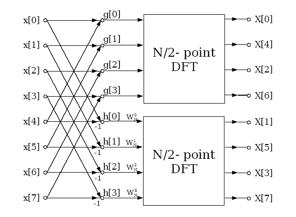
Thus
using 2 MPI processes a distributed memory FFT of length 8 can be
performed by distributing the data such that process 0 has elements
0-3 and process 2 elements 4-7. The two processes then send their
data to each other which is combined as described above, and then
finally a library routine is called to perform the final FFT which is
completely local to the process. This divide and conquer method can
obviously be generalised to any power of two number of processes
calculating an FFT which is of length a power of 2; in general for P
processes there will be Log2(P) stages where data is
exchanged and combined by pairs of processes, and then each of the
processes will perform a length N/P serial FFT by use of a standard
library routine.
It can
also be seen that the data distribution in the above is the 1
dimensional analogue of the domain decomposition used by DL_POLY. The
generalisation of the above to 3 dimensions is clear. The processors
are split into a Px*Py*Pz grid (“the
processor grid”), the parallel 1D transforms in the x direction are
all performed at once, and this is repeated for y and z. This results
in a FFT algorithm that precisely matches that required by DL_POLY
and therefore avoids any initial or final data redistribution. It is
this method that I earlier implemented. The resulting code, the
Daresbury Fourier Transform (DaFT), was then used by DL_POLY_3.
The
only apparent problem is the vectors produced by the DIF method are
not in natural order; it is in so called “bit reversed” order,
and to return it to natural order would require extensive
communications so apparently defeating the point of the exercise. In
fact for DL_POLY_3 and DL_POLY_4 this is not an issue because the
operations required in Fourier space are, as noted above, local.
As a result the operations in Fourier space can be performed very
easily in bit reversed order as all that is required to be known is
the value of m
for the grid point under consideration, and in particular it is not
necessary to know the value on the grid for any other vector m',
thus obviating the need for any communication.
Further if the inverse Fourier transform required for the calculation
of the forces is performed by the Cooley and Tukey algorithm, a
decimation in time (DIT) algorithm, and the input values are provided
in bit reversed order, the final result is returned in the natural
ordering in real space. The graphical representation of the DIT
method is
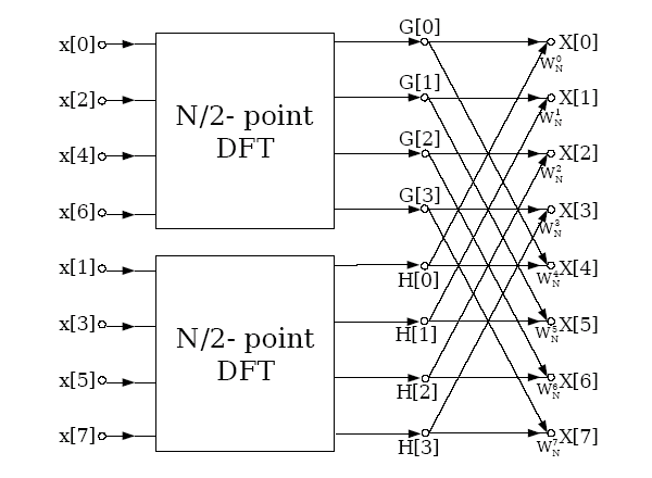
It
can be seen that in parallel a very similar method to that employed
for the forward transform can be employed, except the data exchange
and serial FFT steps are reversed. Further because the inverse
transform takes its input in bit reversed order no communication is
required between the two FFT stages.
The
resulting code performs very well, and it was shown in xiv
that while as a stand alone routine it is often slower than the
standard slab based 3D FFT methods, in DL_POLY_3 DaFT was almost
always superior within DL_POLY due to the extra communications that
slab based methods require to bring the data into the appropriate
distribution.
However
the code as described above is limited to process counts that are
powers of 2. As at large processor counts the separation between
neighbouring powers of 2 increases this restriction can result in the
scientist having to markedly “scale up” his computational system
simply so that he or she can run on the next lowest power of 2 cores,
so resulting in an appreciable increase in cost of the calculation.
This is a waste of their computational budget. Further with HECToR
phase2a for the first time the nodes themselves were not powers of 2,
forcing the scientist to under-populate at least 1 of the nodes in
most runs. As HECToR accounting is “by the node” this was another
waste of computational resources. Both these above points led to the
current work, to remove the above restrictions.
On the
other hand it should be noted that the dimensions of the FFT grid, as
opposed to the processor grid, are not
restricted to powers of 2. Rather the dimensions are restricted to
the values PμNFFT,
where Pμ
is the number of processors down a given dimension (x,y or z) of the
processor grid, and NFFT
is a length which the serial FFT library routine can perform. In
other words the restriction is that the length must be a multiple of
the number of processors, and the allowed multiples are determined by
the capabilities of the serial FFT library function. In practice the
GPFA routines of Tempertonxv
are used. These can perform FFTs for sequences whose lengths have
prime factors 2, 3, or 5. Thus DaFT in its original formulation was
capable of 3 dimensional parallel FFTs where the dimensions of the
FFT had length Pμ*2a*3b*5c,
for zero or positive integer a, b and c and Pμ
a power of 2. However DL_POLY_3 imposed the restriction that the
dimensions of the FFT grid must be a power of 2, a point I shall
return to when describing the current work.
Thus
the overall 3D DaFT algorithm is actually very simple, in many ways
much simpler than the standard “transpose” based methods. Given a
processor grid of size Px*Py*Pz
and an FFT grid of size Nx*Ny*Nz
Perform
the 1D FFTs in the x direction. Each of these are split over Px
cores, and each core has (Ny/Py)*(Nz/Pz)
of these to perform, and obviously only one message need be sent for
all the 1D FFTs at each stage, thus ensuring long messages
As
1 but for the y direction
As
1 but for the z direction
Thus
to be effective it is necessary only to achieve good scaling of the
1D FFTs to approximately P1/3
cores, where P is the total number of cores used by the job, since
each 1D FFT is only distributed across ~ P1/3
cores.
4 DaFT (Mixed Radix)
The
major limitation on DaFT is that it limited to powers of 2 number of
processes, a limit that is not commensurate with either some modern
computational systems or the needs of some users of DL_POLY. Thus for
DL_POLY_4 work has been funded by the dCSE mechanism to provide a
generalisation of the above. The original proposal was to allow
process grids which had factors of the form 2a*30-2*50-1,
this form being chosen to
Fit
the architecture of the then current phase2a HECToR system which had
24 core nodes
Allow
some future proofing to possible future architectures
Allow
sufficient flexibility to the scientist so that waste of
computational resources due to using “oversized” systems was
markedly reduced.
In
fact what was implemented was a full mixed radix domain decomposed
parallel
FFT. This allows for any
number
of processes to be used for the FFT, though due to the nature of the
both the algorithm and implementation it is most efficient if the
prime factors of the number of processes used be small integers.
The
mixed radix algorithm depends upon the following identity: If the
length of a Fourier Transform is N and it can be factored as N=N1*N2
then
can
be written in terms of the two factors as
It
can be see that again the Fourier transform has been decomposed into
2; the term in parentheses is an FT of length N2,
while the outer sum is an FT of length N1
with some extra phase (“twiddle”) factors. Thus each of the two
FTs could be calculated by the parallel DIF algorithm described
above, generalising it where necessary to deal with the case where 2
is not the factor of interest.
However
in practice to deal with a general number of processes efficiently
would be somewhat complicated by this method as the communication
patterns depend fundamentally on the value of the prime factor of
interest. Instead the pragmatic decision was made to split the
factors into two sets, short and long.
Short factors are small primes, and thus the factorisation of the
number of processors will typically contain these factors raised to
high powers. As such these are performed by either a DIF or DIT FFT
algorithm, depending on the direction of the transform. Long factors
are larger primes, and thus they will be (typically) raised to low
powers in the factorisation. In this case the FFT algorithm often
gives little gain compared to a simple, straightforward quadrature
based discrete Fourier transform (DFT - in fact if the power is unity
the DFT and FFT are identical), and as such the longer factors are
all amalgamated and a single DFT is performed. Currently the only
short factor supported is 2, but the code has been designed to allow
easy addition of other primes numbers to this set.
To
clarify the above consider the case where the 1D FFT in a given
direction is being performed by 36 cores. As 36=22*32
the short factors are 2, and will use the distributed FFT algorithm
outlined above, while the long factor is 32=9,
and this FT associated with this factor will be performed by a simple
DFT.
In
the above equation the long factors correspond to the summation over
j2,
while the short factors are the j1 sum. Thus the
method for the mixed radix forward transform is
Perform
the DFT for the long factors
Scale
with the appropriate twiddle factors
Perform
the FFT for the short factors
To
perform the DFT the data has to be circulated amongst the processors
that hold the DFT of length N2. If the factorisation of
the number of processors along the dimension is Pμ=S*L,
where S is
the product of the short factors and L the same for the long, then
there will be S of these transforms, and each of these transforms
require the data to be communicated between the L processes that hold
the data for it. A number of different ways of performing this data
circulation were investigated, but the in practice a simple systolic
loop with double buffering was found most effective. This is possibly
because it allows some overlap of computation and communication as
can be seen from the code excerpt below:
which
= 0
work = a
a = 0.0_wp
rank =
desc%rank; rem_rank = rank
Do pulse = 0,
desc%size - 1
t = Exp(
Cmplx( 0.0_wp, &
( sign *
2.0_wp * pi * rank * rem_rank ) / desc%length, Kind = wp ) )
If ( which ==
0 ) Then
If ( pulse
/= desc%size - 1 ) Then
Call
MPI_IRECV( work2, 2 * Size( work2 ), wp_mpi, down, down, &
desc%comm,
comms_request1, comms_error )
Call
MPI_ISEND( work , 2 * Size( work ), wp_mpi, up, rank, &
desc%comm,
comms_request2, comms_error )
End If
a = a + t
* work
If ( pulse
/= desc%size - 1 ) Then
Call
MPI_WAIT( comms_request1, comms_status, comms_error )
Call
MPI_WAIT( comms_request2, comms_status, comms_error )
End If
Else
If ( pulse
/= desc%size - 1 ) Then
Call
MPI_IRECV( work , 2 * Size( work ), wp_mpi, down, down, &
desc%comm,
comms_request1, comms_error )
Call
MPI_ISEND( work2, 2 * Size( work2 ), wp_mpi, up, rank, &
desc%comm,
comms_request2, comms_error )
End If
a = a + t
* work2
If ( pulse
/= desc%size - 1 ) Then
Call
MPI_WAIT( comms_request1, comms_status, comms_error )
Call
MPI_WAIT( comms_request2, comms_status, comms_error )
End If
End If
which = Mod(
which + 1, 2 )
rem_rank =
Mod( rem_rank + 1, desc%size )
End Do
The
algorithm described above will work for any number of processors
provided the length of the 1D FFTs in each direction is a multiple of
size of the processor grid in the corresponding dimension. For
DL_POLY_4 in practice this is not an issue. The user input that
determines the grid size is a minimum accuracy for the SPME method.
As increasing the FFT grid size increases the accuracy of the SPME
method, it is therefore sufficient to simply increase the grid size
until both the accuracy criterion and the above restriction are
satisfied. In practice the overhead is small; the cube root of the
number of processors on HECToR is roughly 35, thus indicating that in
a bad case the FFT grid is 34 bigger than necessary in each
direction. Compare this to a factor of 2 for the previous version! As
a job on so many cores would have a grid of the order of 1000s in
each of the 3 directions the overhead is obviously small.
5 Other Changes
After
the FFT was generalised to deal with arbitrary numbers of processes
it was necessary to do the same for DL_POLY. Earlier version of the
application assumed
The
number of cores was a power of 2
The
dimensions of the FFT grid were powers of 2
The
former is the major restriction, once it is removed the later follows
naturally; indeed the general procedure is described in the previous
section, namely to pick a size that satisfies the minimum accuracy
criterion and then increase it until the dimension was consistent
with the requirements of the new DaFT routines.
The
removal of restriction 1 required a number of changes to code. By far
the largest of these was to implement an algorithm to determine the
domain decomposition for an arbitrary number of processes. For a
given number of cores the chosen decomposition should
Enable
DL_POLY to run as efficiently as possible
Reproduce
the results of earlier versions of the code where appropriate
To develop such
an algorithm note that
Just as for
halo exchange codes the time spent in message passing is
proportional to the surface area of the parallelipipeds into which
the unit cell is decomposed
For a given
process count the volume each process holds is constant,
irrespective of the decomposition
Therefore as
to maximise efficiency one has to minimise the ratio of surface area
of the parallelipipeds to their volume, the problem reduces to
finding that decomposition which minimises the surface area of the
parallelipipeds
Thus the problem
reduces to an optimisation. There are, however, two slight
complications when different decompositions can result in the same
surface area. This can occur due to symmetry of the system, e.g. on
16 processors with a cubic unit cell 4*2*2, 2*4*2 and 2*2*4
decompositions all obviously give the same surface area for the
parallelipipeds. However it can occur for more general cases where no
such apparent symmetry exists. To choose a decomposition in such
“degenerate” cases the new code
Chooses the
factorisation which minimises the maximum number of cores along any
dimension in the process grid as this should maximise the efficiency
of DaFT
If 1 does
not remove all degeneracies choose the case such that Px≥Py≥Pz.
This ensures that results from earlier versions of DL_POLY are
reproduced
Thus the full
algorithm for choosing the decomposition for P cores is
6 Testing and
Verification
The
new code was verified against all the standard DL_POLY test cases
found at xvi
and also a number of supercells of Sodium Chloride. In all cases when
run on powers of two cores the results from the earlier versions of
the code were reproduced. For cases that were not on powers of 2 the
calculated thermodynamic properties of the system were the same as
those calculated for runs on powers of 2.
7 Benchmarking
The
new code was benchmarked by studying NaCl with a system comprising
216,000 ions and run for 2000 time steps. This is a sufficient number
of steps to minimise the effect of the start up and close down time.
Configuration dumping was also turned off. The time taken for
studying such a system is dominated by the electrostatics, and so it
is ideal for studying the effect of this work. In particular the
major concern was that the performance of the code may be
significantly degraded when the processor grid was not a power of 2.
Figure 1
: Performance of the new code
Figure 1 shows
the performance, measured as MD time steps per second:
The
two curves are for those runs that are on powers of two (in red) and
those that are not (in
blue). It can be seen that there is little difference in the two
curves. Thus the concerns about the efficiency on non-powers of 2
were unwarranted.
Table
1 shows the raw numbers used to generate the above curves, along with
the prime factorisations of the number of cores
-
|
Cores
|
Prime factorisation
|
Timesteps/s (non power of 2)
|
Timesteps/s (power of 2)
|
|
24
|
23*3
|
2.08
|
|
|
32
|
25
|
|
2.8
|
|
40
|
23*5
|
3.19
|
|
|
48
|
24*3
|
3.98
|
|
|
64
|
26
|
|
5.19
|
|
72
|
23*32
|
4.87
|
|
|
96
|
25*3
|
6.76
|
|
|
120
|
23*3*5
|
7.93
|
|
|
128
|
27
|
|
9.1
|
|
160
|
25*5
|
10.8
|
|
|
192
|
26*3
|
12.34
|
|
|
216
|
23*33
|
13.65
|
|
|
256
|
28
|
|
15.85
|
|
288
|
25*32
|
15.82
|
|
|
384
|
27*3
|
20.72
|
|
|
512
|
29
|
|
24.48
|
|
768
|
28*3
|
31.18
|
|
|
1024
|
210
|
|
36.02
|
|
1536
|
29*3
|
38.84
|
|
|
2048
|
211
|
|
44.01
|
Table 1
: Performance of the new code
It
can be seen that factorisations involving low powers of 3 and 5 are
very effectively dealt with by the new routines, and certainly the
initial aim of core counts that factored as 2a*30-2*50-1
has been more than met.
The
new code has been released to users, and is part of the standard
release of DL_POLY_4.
8 Conclusion
A
new multi-radix parallel FFT has been implemented within DL_POLY_4.
Like the
old FFT this fits exactly the same domain decomposition that
DL_POLY_4 uses, but is not restricted to using powers of 2 number of
cores. This new flexibility has been shown to come at little
performance penalty, and thus the new code both better fits modern
multicore architectures, such as HECToR phase 2, and also allows the
scientist to study the system of interest without having to
artificially inflate it to fit the restrictions of the code.
This
project was funded under the HECToR Distributed Computational Science
and Engineering (CSE) Service operated by NAG Ltd. HECToR A Research
Councils UK High End Computing Service – is the UK’s national
supercomputing service, managed by EPSRC on behalf of the
participating Research Councils. Its mission is to support capability
science and engineering in UK academia. The HECToR supercomputers are
managed by UoE HPCx Ltd and the CSE Support Service is provided by
NAG Ltd. http://www.hector.ac.uk.
ii http://www.ccp5.ac.uk/
iii
I.T. Todorov, W. Smith, K. Trachenko & M.T.Dove, J. Mater.
Chem., 16, 1911-1918 (2006)
iv
I.J. Bush, I.T. Todorov and W. Smith, Comp. Phys. Commun., 175,
323-329 (2006)
v
M.R.S. Pinches, D. Tildesley, W. Smith, 1991, Mol Simulation, 6, 51
vi P
Ewald, Ann. Phys. 64 (1921) 253.
vii J.
Perram, H. Petersen and S. De Leeuw, Mol. Phys. 65 (1988) 875.
viii
D. Fincham, Mol. Simulation 13, (1994), 1
ix U.
Essman, L. Perera, M.L. Berkowitz, T. Darden, H. Lee, L.G. Pedersen,
J. Chem. Phys. 103, 19, (1995)
x J.W.
Cooley, O.W. Tukey, Math.
Comput. 19, 297-301, (1965)
xi I.J.
Schoenberg, “Cardinal Spline Interpolation”, Society for
Industrial and Applied Mathematics, Philadelphia, PA, (1973)
xiv I.J.
Bush, I.T. Todorov and W. Smith, Comp. Phys. Commun., 175, 323-329
(2006)
xv C.
Temperton, J. Comp. Phys. 52, 1, (1983)
xvi ftp://ftp.dl.ac.uk/ccp5/DL_POLY/DL_POLY_4.0/DATA/