A load balancing algorithm

for Molecular Dynamics simulations

Laurence J. Ellison, 10th May 2011

Abstract

This report describes a prototype load balancing algorithm designed to improve the efficiency of molecular dynamics simulations, specifically those in which the system under study is characterised by large spatial variations in atom density. At root the parallelisation scheme used in the load balancer is similar to the widely used domain decomposition scheme, however each domain is further subdivided into a number of cells. The coordinates of the atoms within cells can be reallocated from processors with a heavy work load to ones with more modest work loads to effect a more even work distribution.

The prototype load balancing algorithm is based around a rudimentary MD time stepping loop in which only 2-body interactions are considered and the atom trajectories are non-physical. The intention here was to provide a simple framework on which to develop and test the basic algorithm. The results of performance tests carried out on HECToR are encouraging, with good speed ups observed for a number of simple test systems. The largest test run consisted of some 5 million atoms run on a maximum of 2744 cores.

The prototype load balancer code as it stands provides a good basis for understanding how the performance of the algorithm is affected by various operational parameters. However further work is necessary to integrate the algorithm into DL_POLY_4, a long standing, general purpose MD package with a wide user base. This is the ultimate aim of the project and the ultimate test for the load balancing algorithm. If this can be achieved it is hoped that the improved performance conferred by the load balancing will enable users to obtain results in a shorter time frame and to make better use of the resources on which they run their jobs.

Contents
1.	Introduction.................................................................................... 2
2.	Code overview ............................................................................... 3
3.	Performance test results ............................................................... 9
4.	Further work ................................................................................ 15
5.	Summary and conclusions ........................................................... 17
	Appendix � Performance test data

1. Introduction

In molecular dynamics (MD) simulations parallelised using the domain decomposition (DD) scheme, the simulation volume, which we refer to as the MD cell, is divided into a number of spatial domains of equal size, each one being allocated to a particular core^* on the machine on which the simulation is run. The work load for each core consists of two main components: (i) the calculation of the forces acting on the atoms within its domain and (ii) the message passing necessary for importing additional atomic coordinates from neighbouring cores as required to complete those force calculations. If the distribution of atoms within the MD cell is more or less uniform, then each core should have roughly the same work load � the work loads are said to be balanced. If however the atom distribution becomes significantly non-uniform, as in figure 1(a), then we may well find that certain domains contain large numbers of atoms whilst others are relatively sparsely populated. The effect of this will be that cores responsible for regions of high atom density will have large work loads whilst those responsible for the sparse regions will be largely idle for much of the time. There are two major disadvantages here, firstly the MD simulation will only run as quickly as the slowest core participating, therefore the average step time and thus the time to solution will be dictated by the core with the heaviest work load. Secondly the available hardware is not being utilised as efficiently as it might be since many of the cores are doing very little work.

Figure 1.

(a) Schematic representation of the MD cell partitioned into domains, the shaded disk represents a highly non-uniform atom distribution. (b) The basic strategy on which the load balancing algorithm is based is to subdivide each domain into cells and reallocate cells from cores responsible for densely populated domains to to cores responsible for domains containing fewer atoms.

The prototype load balancing program that we have developed seeks to ameliorate this situation by reallocating atoms from busy cores to less busy ones. In order to do this each domain is subdivided into a number of cells each of the same size (figure 1(b)). Periodically, within the MD time stepping loop, each core estimates its overall work load as a function of the current atom distribution. The work loads are then pooled via global communication and if at this point there is sufficient imbalance in the work loads, cells are transferred from busy cores to less busy ones. By the transferal of a cell, we mean that all the atoms within that cell are allocated to another core which then becomes responsible for calculating the forces on the atoms in that cell. Cell transfer continues until the work loads are balanced within a desired tolerance. This should result in a speedup of the simulation, i.e. we should observe a reduction in the average time step length as compared to the equivalent test run without load balancing. Furthermore all the cores should be engaged in doing work for the majority of the simulation time. A successful load balancer therefore allows the user to obtain results in a shorter time frame and makes more effective use of the hardware available.

The primary objectives of this project were (i) to develop a prototype load balancer designed to improve the performance of parallel MD simulations, (ii) to thoroughly test the load balancer and understand the effect of the various operational parameters on its performance and (iii) to incorporate the load balancing algorithm into the latest release of the general purpose MD package DL_POLY_4, which uses the DD method of parallelisation but does not currently feature any load balancing functionality. We have succeeded in developing an algorithm that is robust and flexible, in particular the cell and domain dimensions can be selected completely independently of the cut-off distance for atom-atom interactions. The code has been exhaustively tested for errors and the results of the performance tests are encouraging. In a number of these tests the load balancer achieved a speedup close to the theoretical maximum and very rarely did the load balanced version ran slower than the control test. In other words it appears that in most circumstances there is little to be lost by deploying the load balancer but potentially much to be gained in terms of efficiency. Unfortunately, in the time available, it was not possible to integrate the load balancing algorithm into DL_POLY_4. Both codes are complex in their own ways and so the task of incorporating the one into the other is highly non trivial. Moreover unforeseen design issues did arise in the latter stages of the load balancer development that demanded attention and it was deemed more important to make sure that the prototype was, as far as we could be sure, bug free and operating as efficiently as possible rather than rushing to integrate a defective prototype into DL_POLY_4 prematurely. However some preliminary has been done to outline how the integration might be implemented.

The remainder of this report is divided into four further sections, in section 2 we will give an overview of the architecture of the load balancer code. Section 3 will present the results of some of the performance testing that was carried out. In section 4 we discuss weaknesses in the existing code and steps that might be taken to improve its effectiveness. Section 5 summarises and draws conclusions from the work presented in the earlier sections.

2. Code overview

The load balancer source code is written in Fortran 90 and message passing is implemented using MPI calls. A serialised version of the source code has been put through the Forcheck application on the NAG CSE machine, softeng.cse.rl.ac.uk to check for compliance with the F90 standard and weed out dubious programming practices. In terms of organisation the top level program consists of three stages presented in summary form in figure 2.

In stage 1 the preliminary steps common to many simulation codes are performed such as the allocation of permanent arrays, definitions of constants, reading of user defined directives from an input file and setting up of the initial atom configuration. We will not go into the details here, a comprehensive overview of the top level subroutines that implement these steps can be found in the documentation that accompanies the source code. In addition the header and embedded comments in each subroutine provide further detail.

Stage 3 of the program is primarily concerned with the output of diagnostic data. The diagnostics include checks of global cell and atom tallies, local and global time averages for each primary subroutine (useful for inferring bottlenecks and disparities in work load) and also the amount of memory allocated to the major dynamic arrays used by the program.

The meat of the code is located within stage 2, the time stepping loop where the bulk of the communication and computational work is done. The role of each major block of code in the time stepping loop will now be outlined

Program Main

Stage 1: Preliminaries

Initialise MPI

Make preliminary definitions

Open diagnostic files

Read user input file

Setting up the initial atom configuration

Construction of domain and cell maps and neighbour lists

Allocation of permanent bookkeeping arrays

Partitioning of the MD cell into domains

Subdivision the domains into cells

Stage 2: Time stepping loop

Do nstep=1, num_steps, 1

Get required cell populations in order to determine initial load imbalance

Load balancing � i.e. reallocation of cells if work loads are sufficiently imbalanced

Get locations of cells required for local forces calculations

Import atoms required for local force calculations

Calculate total forces acting on on-core atoms

Export opposite force components acting on off-core atoms

Atom translations

Reallocate atoms that have crossed cell boundaries to their new cells

Check local cell and atom tallies

Optional measurement of ρ (a parameter used in the work load estimate) from timing data

Option to restore all cells to their original cores

Wind up current time step

End Do

Stage 3: Wind up simulation

Check global cell and atom tallies

Output diagnostic data

Deallocation of permanent arrays

End Program Main

Get required cell populations in order to determine initial load imbalance

The estimate of the relative overall work load, W, on each core is given by the following formula:

W = W₁ + ρW₂ (1)

Here W₁ is the number of 2-body interactions that need to be evaluated by that core and W₂ is the number of atom coordinates that need to be imported from other cores to complete the 2-body force calculations. The parameter ρ is the ratio of the average cost of importing a single atom to the average cost of evaluating a single pair interaction. The calculation of W is made separately on each processor then, at the start of the load balancing subroutine, the results are pooled and the global work distribution thus obtained.

Now in order to perform the work load calculation, the local core must know the populations of each of its required cells. The term required cell has a specific meaning that derives from the way 2-body interactions are calculated in the prototype load balancer. Consider two atoms i and j located in cells A and B respectively which are within the cut-off distance of one another as shown in figure 3(a).

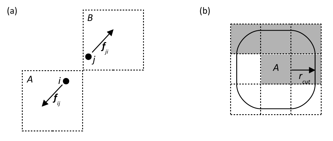
The force on j due to i is equal and opposite to the force on i due to j. Therefore we can choose to calculate only the force component f_ij and simply add the opposite of this, f_ji = -f_ij, to the net force on j. The upshot of this is that to complete the force calculations for the atoms in a given 'central' cell, we do not require the coordinates of the atoms in all the surrounding cells within the cut-off of that cell, only those within a 'semi halo' as it were, as shown in figure 3(b) � these are the so called required cells.

Now some of the required cells for a given central cell allocated to a particular core may well be allocated to a different core � they are said to be off-core. The coordinates of atoms within required cells that are off-core will therefore need to be imported. Given that load balancing causes cells to be arbitrarily moved from core to core, the task of finding out which core a particular cell is located on and the subsequent acquisition of the coordinates of the atoms within that cell presents special difficulties. The strategy used to solve this problem is to periodically update the home core (the core responsible for the domain on which a cell is physically located) with information about its so called native cells i.e. cells physically located on that core's domain. The type of information that needs to be stored on home cores is typically the current hosts of its native cells (the core they are currently allocated to) and their populations. Any core requiring information about an off-core cell, wherever it may be located, contacts the home core of that cell to acquire it. This 'forwarding address' paradigm is predicated on the fact that although a cell could be allocated to any core in the system, given the identity of the cell (specified within the code by a unique global index) its physical location and therefore its home core can always be determined. A scheme based on this idea is used to furnish the required cell populations. The details of the scheme are too detailed to go into here although further details are contained in the documentation accompanying the source code. A crucial aspect of this scheme that should be mentioned however is that it the transfer of information within it is accomplished by highly selective point-to-point message passing. This sort of efficiency is essential if the benefits of load balancing are not to be outweighed by the extra communication overheads entailed by moving data off local cores. Similarly global communications must be kept to a minimum because their use is likely to undermine the scalability of the algorithm.

Load balancing

Having obtained the populations of its required cells, each core now makes an estimate of its overall work load. The workloads of all cores are then pooled via a global summation and each core calculates the mean and standard deviation of this work load distribution. If the ratio of the standard deviation to the mean is above a desired threshold then load balancing is implemented. The first step in performing load balancing is to rank the cores in descending order of work load. The busiest cores are then paired up with the least busy cores. Within each of these partnerships, the busy core sends a single cell to the less busy one. Each core then reassesses its work load (taking into account of the redistribution of atoms that has occurred as a result of the cell transfer) and the two partners share this information. If the ratio of the difference between the two partners' work loads to their average work loads remains above a specified threshold then another cell transfer occurs. This procedure is repeated until the required balance is reached between the two partners at which point the load balancing loop is terminated for these two cores. Usually, within a single round of load balancing, in a given time step, this will only result in the balance of work loads between each pair of partner cores. However after several rounds of load balancing, in which a different set of partnerships is set up, the work load distribution will tend to become balanced globally.

Get locations of cells required for local forces calculations

Before the force calculation loop can proceed each core needs to import the cell data required to evaluate all of its pair interactions. In an ordinary (non load balanced) DD based MD simulation, this is achieved by each core receiving halo data from the cores responsible for domains adjacent to its own domain. But if load balancing has been implemented and hence cells transferred away from their home cores, this is no longer sufficient. A core can no longer assume that the atoms it requires are in the possession of the halo cores, it is therefore necessary for it to determine which cores currently host the cells it requires and to request the coordinates of these cells' atoms from those hosts. A specialised scheme based on the forwarding address paradigm described earlier and similar to the one used to acquire cell populations is implemented to achieve this. Again, the details of the scheme are too complex to relate here, but the result of it is that each core acquires the current locations of its required cells from the home cores of those cells. In the course of this procedure the home cores also inform the host cores of how many requests for cells they can expect to receive. This is essential since without this information the host cores will not know how many receives to post to accommodate all such requests. The anticipation of the numbers of messages that cores can expect to receive was in fact the most challenging aspect of the program design.

Import atoms required for local force calculations

At this stage then, each core in its capacity as a client (a term loosely used to describe a core that is requesting information) knows where to acquire its required cells and in its capacity as a host knows how many requests to expect from other cores requesting their required cells. The required atom coordinates are imported and the force loop proceeds.

Calculate total forces acting on on-core atoms

Within the forces calculation loop as it stands, only 2-body interactions in the form of a 12-6 Lennard Jones potential are evaluated. Clearly this falls well short of the functionality of a multi-purpose MD code, such as DL_POLY_4, with its plethora of both inter- and intra-molecular interactions. The justification for this is that to develop a load balancing algorithm from scratch that incorporated the full gamut of molecular interactions would have been an extremely complex task and certainly very much more difficult to debug. Therefore this prototype program was developed with only as much functionality as was considered sufficient to demonstrate that (i) the algorithm is technically robust and (ii) it has the potential to be able to improve the efficiency of more realistic MD simulations. The forces loop even in its current rudimentary state should provide a reasonable representation of the level of computational work load that cores have to contend with in MD simulations. In other words it provides a reasonable basis for testing the performance of the load balancing algorithm.

Export opposite force components acting on off-core atoms

Recalling the earlier discussion of the concept of required cells, following the force calculations it is necessary for the equal and opposite force components acting on atoms whose coordinates were imported to be sent back to the cores from whence they came. This completes the evaluation of the net forces acting on each atom in the system.

Atom translations

In an MD simulation proper the next stage after the forces loop would be for each core to integrate the equations of motion for the atoms allocated to it. We do not do this here, instead simple arbitrary translations are applied to the atoms, there is the option to apply random displacements in randomly chosen directions or to move each atom by a fixed distance along a specified direction. Again the justification for this rudimentary approach is that the purpose of this program is not to perform fully fledged molecular simulations, rather it is to provide a test bed for the load balancing algorithm. The facility for setting up model configurations and evolving them in simple, controllable ways is part of that process.

Reallocate atoms that have crossed cell boundaries to new cells

Ordinarily, following atom translations in DD based MD simulations, atoms only have to be reassigned to different cores when they cross domain boundaries. These cores will always be the ones responsible for the adjacent domains. However if cells have been transferred away from their home cores, as they have when load balancing has been implemented, any atom that crosses a cell boundary must be considered a candidate for reassignment since the neighbouring cell into which it has moved could currently be allocated to any core on the machine. To account for this we again have recourse to a scheme closely related to the 'forwarding address' paradigm. Essentially what happens is that each home core acquires the coordinates of all the atoms that have crossed the boundaries of its native cells (cells that are physically located on the home core's domain). Some of these atoms, as well as crossing cell boundaries, will have crossed into the domains adjacent to the home domain. The home core sends the coordinates of such atoms to the appropriate adjacent domain. Each home core then sends out any atoms that now happen to lie on any of their absent cells (native cells that were reallocated to other cores by the load balancer) to the current hosts of those cells. In this way each core acquires the complement of atoms that, following translations, are physically located on the cells that are currently allocated to it.

Check local cell and atom tallies

In order to make sure nothing has gone awry in the bookkeeping procedures used to move cell data around the system and keep track of its whereabouts, certain tallies and data fields are checked to ensure consistency in the information they contain.

Optional measurement of ρ from timing data

Recall that the variable ρ is the ratio of the average cost of importing a single atom to the average cost of evaluating a single pair interaction. In most of the testing work carried out, the value assigned to this variable was, if truth be told, simply an arbitrary guess. In the earlier stages of the code development, assigning an accurate value to it was not regarded as being overly critical since typically the estimated number of pair interactions in equation (1) dwarfs the number of atoms to be imported and thus the load balancing is dominated by the former term. Thus a reallocation of cells resulting in approximately the same numbers of atoms on each core generally resulted in a reasonable load balance. Nevertheless it would clearly be preferable to obtain a more accurate value for ρ and thus a better work load estimate. With this in mind, in the latter stages of the code development, attempts were made to obtain an empirical value for ρ based on timings of the subroutines in which atoms coordinates are imported and forces exported (before and after the forces loop) and the timing for the forces loop itself. Thus an empirical value of ρ was calculated as follows

ρ_measured = <import cost>/<pair cost>

where the average cost associated with the import of an atom coordinate and the subsequent export of the corresponding equal and opposite force to the host of that atom is given by

<import cost> = (t_{import atoms} + t_{export forces}) / N_imports

where t_{import atoms} is the time spent in the subroutine responsible for importing atoms, t_{export forces} the time spent in the subroutine which exports forces and N_imports is the number of atoms imported.

The average cost of evaluating a pair interaction is given by

<pair cost> = t_forces / N_pairs

where t_forces is the time spent in the forces loop and N_pairs is the number of pair interactions evaluated within the loop.

The intention was to use ρ_measured in the load balancing subroutine in the proceeding time step, with the aim of obtaining a more accurate estimate of the core work load and thus a more effective data distribution across the hardware. Unfortunately it was found that the timings for the import atoms and export forces subroutines were subject to large fluctuations both from time step to time step and from core to core. When the measured value was fed into the work load estimate calculation, it almost always resulted in a worsening of performance, presumably due to some form of feedback mechanism e.g. if for some reason at a particular time step the value of t_{import atoms} happens to dramatically increase, then in the next time step the relative cost of importing atoms will be overestimated and the load balance skewed as a result. As a result, in the performance tests carried out, we had no option but to keep using a reasonable guess for ρ in the work load estimation.

Option to restore all cells to their original cores

This procedure has two purposes, firstly it obviously enables us to reverse the effects of load balancing. This would be particularly useful if the system of interest is initially non-uniform in its atom distribution but in time evolves into one that is more or less isotropic. Secondly it provides an opportunity for a very robust check that the load balancer has operated without error. After all cells have been returned to their home cores, a check of their coordinates at this point should show that they all lie within the bounds of the domain associated with that core. Any exceptions to this would indicate that at some point atom data had been allocated to the wrong cell and/or core.

Wind up this step

To conclude each time step, temporary arrays allocated for the current time step are deallocated. Also the total time taken for the step is measured and the average step time accumulated, clearly the average step time is the primary observation by which we assess the effectiveness of the load balancer.

3. Performance test results

We now present the results of performance tests of the load balancer under various conditions. There are a rather bewildering range of parameters that may effect how the load balancer performs. On the one hand we have the physical properties of the MD system under consideration: its degree of inhomogeneity in terms of atom density, the total number of atoms in the system, the computational demands of the particular interaction(s) between the atoms, the cut-off distance(s) for the interaction(s). Then we have the hardware constraints: the total number of processors available as well as the particular characteristics of the processors e.g. the clock speed, bandwidth, latency and cores per processor; the choice of compiler and compiler flags may also be a significant factor. In addition there are what we might term the operational parameters of the load balancer itself such as the choice of cell partitioning, the value of ρ and how finely we want the work loads to be balanced. In an MD simulation proper some of these would be predetermined such as the potential cut-off, however for the purposes of testing the code we are free to choose any values within reason. It would be a huge undertaking to explore this parameter space exhaustively, so here we confine ourselves to a few simple types of initial atom configuration, systematically alter the number of cores on which these systems are run and also repeat the tests for a number of different cut-off values.

In all tests, the principal measure of performance is the speed-up i.e. the ratio of the average step time for a run carried out without load balancing to the average step time for an equivalent with load balancing switched on. All tests reported here were carried out on HECToR Phase 2b (XE6) processors on 14-18/03/2011. Note that each XE6 processor has 24 cores. The source code was compiled and linked using the PGI compiler with the flags -O3 and -fastsse (the same as the flags used for compiling DL_POLY_4 on HECToR). In all tests ρ was set at a value of 25.0. The tolerance for the load balance � the target value for the ratio of the difference between the two partners' work loads in the load balancing subroutine to their average work loads � was set at 0.05. Most of the tests were run for 100 time steps (from time to time the results were checked against those obtained from equivalent longer runs to ensure that 100 steps indeed a long enough test to give representative results).

System 1

In the first set of tests, one octant of the cubic MD cell was occupied with atoms, arranged on a lattice, whilst the remaining volume was completely empty. This is a rather artificial set-up but its simplicity makes it easier to interpret the results of the tests. The volume of the MD cell, V, was systematically increased in direct proportion to the number of cores, P, on which the system was run. The fraction of the MD cell that was occupied thus remained constant at 1/8. The spacing between the atoms in the occupied region was fixed so that the number of atoms in the system also increased in proportion to the system volume. The choice of domain subdivision is completely at the user's discretion and there is no hard or fast rule for the ideal number of cells. However, as a general rule of thumb, we regard domain subdivision of 4x4x4=64 cells or 5x5x5=125 cells as being sensible choices. If the cell mesh is too coarse, then the packets of atom data that are moved from core to core by the load balancer will be too large to permit an even distribution of work loads. If on the other hand the subdivision is too fine then large numbers of cells will need to be reallocated in order to achieve load balance, the undesirable side effect of this is that the atom data, since it is divided into many small packets, will tend to become highly dispersed across the machine and so the communication overhead associated with the acquisition of off-core data will be large and result in poor performance.

The same set of tests was carried out for a number of different cut-off distances, r_cut, for the Lennard Jones pair interaction. The smallest cut-off used was 0.499 arbitrary units (a.u.), just under 2.5 times the atom spacing, which was set at 0.2 a.u. The choice for this minimum cut-off value was based on the fact that typically in MD simulations, the Lennard Jones potential is truncated at around 2.5σ, where σ is the atom-atom separation at which the potential is zero. The potential minimum, which physically corresponds to the equilibrium separation and here equates to the lattice spacing, occurs at a slightly larger separation of 2^⅙σ or ~1.122σ. Thus the smallest cut-off value of 0.499 a.u. corresponds roughly to the minimum cut-off that is likely to be used in a real MD simulation. However other types of interactions that might be active such as metal interactions and certainly electrostatic interactions would have larger cut-offs, for this reason we repeated the tests for larger cut-off values. In this set of tests, no translations were applied to the atoms because, first and foremost, we wished to understand how the load balancer copes with a given unbalanced atom configuration given a particular domain decomposition and cut-off. Having a static configuration makes the interpretation of the results of the tests less complicated. The complete set of parameters used for the System 1 tests are listed in table 1. The timings for the tests with load balancing off and on are tabulated in the appendix at the end of the report, figure 4 shows the resultant speed-ups.

P	8	64	216	512	1000	1728	2744
N	15625	125000	421875	1000000	1953125	3375000	5359375
% volume occupied	12.5	12.5	12.5	12.5	12.5	12.5	12.5
MD cell dimensions/[a.u.]	10.0	20.0	30.0	40.0	50.0	60.0	70.0
Domain decomposition	2x2x2	4x4x4	6x6x6	8x8x8	10x10x10	12x12x12	14x14x14
Domain dimensions/[a.u.]	5.0	5.0	5.0	5.0	5.0	5.0	5.0
Population of occupied domains	15625	15625	15625	15625	15625	15625	15625
Cell subdivision	5x5x5	5x5x5	5x5x5	5x5x5	5x5x5	5x5x5	5x5x5
Cell dimensions/[a.u.]	1.0	1.0	1.0	1.0	1.0	1.0	1.0
Population of occupied cells	125	125	125	125	125	125	125

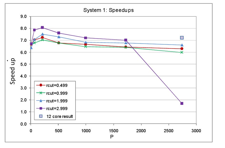
In nearly all the System 1 tests we observe good speed up values in the range of 6.0 to 8.0, the latter value being the theoretical maximum given the 1/8 fraction of the MD cell that is occupied by atoms. The only System 1 test in which load balancing delivers a relatively poor speed up is the one that is run on the largest core count with the largest cut-off. We believe the reason for this anomaly is that in this test the total number of cells into which the occupied region is divided is at its largest � it will be P/8 multiplied by the number of cells into which each domain is subdivided, for the P=2744 system the number of occupied cells will therefore be 343*125=42875. Many of these cells will be allocated to other cores by the load balancer resulting in much dispersion of the atom data. This coupled with the large cut-off will incur a heavy communication penalty in order for cores to import required cells and export forces. The result, we suspect, is that the comms network becomes overloaded before and after the forces loop (where atoms are imported and forces exported), hence the inferior speed-up value. This suspicion was given credence by the fact that when the test was rerun using the same number of cores overall but with the number of cores per processor set at 12 as opposed to the full complement of 24 on each XE6 processor, the speed up rose from 1.68 to 7.12. Presumably the act of running on fewer cores per processor increased the amount of bandwidth available per core thus enabling them to better cope with the heavy communication costs. We note that for all the cut-offs the speed up tends to peak at P=216 but declines slowly with increasing core counts. Again this is attributable to the fact that, in this mode of testing, as we increase the core count the number of occupied cells rises along with the number of cores available onto which they can be moved by the load balancer. As a consequence the atom data tends to become increasingly dispersed across the hardware and the number of communications necessary to acquire off-core data rises.

System 2

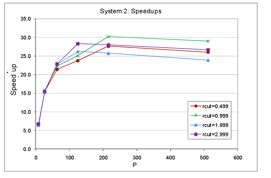
In the second round of performance tests only a single domain was occupied with atoms, the atom spacing was again set at 0.2 a.u. and the atoms were held static. Since only a single domain is occupied, as P and with it the number of domains increases, the fraction of the MD cell containing atoms falls in direct proportion. The domains were again each subdivided into 125 cells. The complete set of parameters used for the System 2 tests are listed in table 2. The timings for the tests with load balancing off and on are tabulated in the appendix at the end of the report, figure 5 shows the resultant speed-ups.

P	8	27	64	128	216	512
N	15625	125000	421875	1000000	1953125	3375000
% volume occupied	12.50	3.70	1.56	0.80	0.46	0.20
MD cell dimensions/[a.u.]	10.0	15.0	20.0	25.0	30.0	40.0
Domain decomposition	2x2x2	3x3x3	4x4x4	5x5x5	6x6x6	8x8x8
Domain dimensions/[a.u.]	5.0	5.0	5.0	5.0	5.0	5.0
Population of occupied domains	15625	15625	15625	15625	15625	15625
Cell subdivision	5x5x5	5x5x5	5x5x5	5x5x5	5x5x5	5x5x5
Cell dimensions/[a.u.]	1.0	1.0	1.0	1.0	1.0	1.0
Population of occupied cells	125	125	125	125	125	125

We find that the peak speed-up occurs at P=125 or P=216 and then slowly declines with higher core counts. This is not so surprising for when the number of cores matches the number of occupied cells available for reallocation, we would not expect any further benefit from increasing the core count since the maximum number of cores that can be allocated a populated cell can never exceed 125. It is not obvious therefore why the peak speed up should occur at P=216 rather than P=125 for the rcut=0.499 and rcut=0.999 systems. Nevertheless the overall message from this set of tests is fairly clear: as the dense to sparse volume fraction of the system diminishes there is relatively speaking less benefit to be had from load balancing, particularly at high processor counts, since in this regime computational work load per processor will be relatively small and in addition the data will tend to become more widely dispersed across the machine.

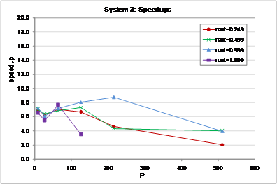
System 3

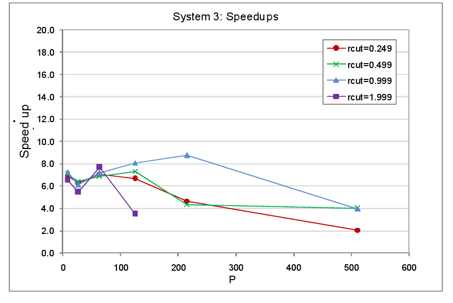
In the third round of performance tests, the system set up was as with System 1, a cubic MD cell with one octant occupied and the remaining volume empty. This time though the physical size of the system was kept fixed whilst the number of cores was increased. The atom spacing was 0.1 a.u. in this set of tests. The number of cells per domain was again 125 and once again the atoms remained static throughout. The timings for the tests with load balancing off and on are tabulated in the appendix at the end of the report, figure 6 shows the resultant speed-ups.

P	8	27	64	128	216	512
N	125000	125000	125000	125000	125000	125000
% volume occupied	12.5	12.5	12.5	12.5	12.5	12.5
MD cell dimensions/[a.u.]	10.0	10.0	10.0	10.0	10.0	10.0
Domain decomposition	2x2x2	3x3x3	4x4x4	5x5x5	6x6x6	8x8x8
Domain dimensions/[a.u.]	5.00	3.33	2.50	2.00	1.67	1.25
Population of occupied domains	125000	37037	15625	8000	4630	1953
Cell subdivision	5x5x5	5x5x5	5x5x5	5x5x5	5x5x5	5x5x5
Cell dimensions/[a.u.]	1.000	0.667	0.500	0.400	0.333	0.250
Population of occupied cells	1000	296	125	64	37	16

The key characteristic of this test set-up is that as the core count increases, the number of atoms per core and per cell falls. This in fact represents a very wasteful use of hardware irrespective of whether or not we attempt load balancing or not. The more cores we throw at this system the lower will be the computational work load per core but at the same time the communication overheads will increase as the cut-off takes in an increasing number of domains and cells. This is reflected by the fact that both for the non load balanced and load balanced tests, the average step time does not decrease significantly beyond processor counts of 100 or so, indeed the step time actually increases for the rcut=1.999 load balanced test. The message here is clear � when setting aside resources for parallel jobs the magnitude of the computational work load that the job entails must always be considered. Much better to run many small system simulations simultaneously on few cores each than to run a single small job on many cores.

System 4

In the final sets of tests we made an effort to set up scenarios more in keeping with a real MD simulation. The test systems consisted of a spherical region of dense atom concentration of radius 1.25 a.u. within a cubic MD cell of size 4.0 a.u. divided into 4x4x4=64 cubic domains of size 1.0 a.u. Thus all tests were run on 64 cores. Note that the volume of the sphere relative to that of the MD cell is approximately 1/8, in other words similar to the value for the single occupied octant set-ups of the System 1 and System 3 tests described earlier. The cell subdivision was also 4x4x4 and thus the cell size 0.25 a.u.

In one set of tests, 'Sphere 1', the atom spacing was set at 0.1 a.u., which resulted in an atom population of 8144 in the spherical region � a relatively small number of atoms for a run carried out on 64 cores. The cut-off used for this set tests was 0.249 a.u. In a second set of tests, 'Sphere 2', the atom spacing was halved to 0.1 a.u. resulting in an atom count of 72327 within the sphere and thus a more substantial computational work load for the hardware. The cut-off used in these tests was 0.1249 a.u. in keeping with the halving of the atom separation. Several additional variations were applied both to the basic Sphere 1 and the Sphere 2 set-ups as follows:

6. The atoms within the sphere remained static and the surrounding volume was devoid of atoms.

7. The sphere was again surrounded by vacuum but each atom within it was moved in the positive x-direction at a rate of 0.01 a.u. every time step. This obviously allows us to see how the load balancer copes when the atoms in the system are moving across cell and domain boundaries en masse.

8. The sphere was static and surrounded by vacuum but the atoms within the sphere were set in random motion with the maximum displacement components per time steps set at 0.10 and 0.05 a.u. for Sphere 1 and Sphere 2 respectively.

9. The sphere of static atoms was surrounded by a sea of randomly placed atoms at a number density approximately 1% that of the number density within the sphere. This is a crude representation of the type of situation we might find in a simulation where a gas has condensed into a droplet of liquid surrounded by a vapour.

10. As (4) but with all atoms in both the sphere and the surrounding 'vapour' subject to the same random motions as in (3).

11. As system (5) but run for a much greater number of steps so that by the end of the run the atom distribution was essentially isotropic.

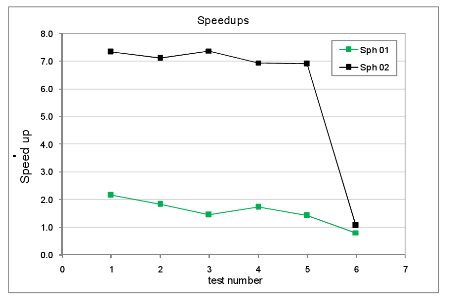
The timings for the tests with load balancing off and on are tabulated in the appendix at the end of the report, figure 8 shows the resultant speed-ups. Comparing the Sphere 1 and Sphere 2 tests we see that the speed-up for the Sphere 1 tests are much lower than for Sphere 2. This reflects the fact that in the former, the number of atoms is relatively small, around 125 per core as opposed to the latter where their are over 1000 atoms per core. As noted earlier, in general the benefits of load balancing will be more pronounced when the computational work load per core is greater.

We also observe that neither the imposition of atom translations nor the presence of a diffuse gas of atoms surrounding the dense spherical region has a marked effect on the speed-ups in either Sphere 1 or Sphere 2 systems. We can therefore be more confident that the load balancing algorithm is likely to perform well under true simulation conditions where atoms are moving and where the density variations are not so clear cut as they were in the earlier tests.

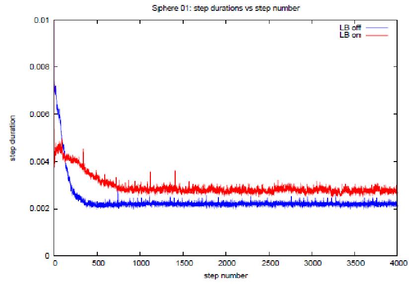
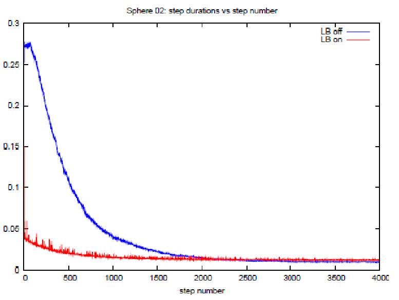
Perhaps the most encouraging results are shown in figures 9(a) and (b). These are graphs of the time step durations plotted against step index for the variant 6 tests in which random atom translations were applied for long enough for the system take on a uniform density^*. By the end of the runs it is true that the step times for the load balanced tests are slightly longer than for the non load balanced runs. This is undoubtedly due to the fact that the load balancing done in the early stages of the test, when the atom distribution was highly non uniform, has resulted in dispersion of the data which persists even when the system has become isotropic. This will inevitably incur additional communication overheads over and above that necessary in the equivalent non load balanced run. However the differences between step timings at the end of the runs are relatively small, this suggests that the residual effects of load balancing need not have severe effects even when the simulation tends towards an isotropic state. More generally, it suggests that the load balancing algorithm is fairly efficient. Furthermore, recall from the the overview of the program in

section 1, that the facility exists within the time stepping loop, at any point, to return all cells to their home processors thus reversing the effects of prior load balancing. It would be fairly simple to automatically check for the emergence of uniformity in the atom distribution (for example by periodically checking globally how many atoms are physically located on each domain) and hence roll back the load balancing at the appropriate juncture. This lends further weight to the belief that, though load balancing inevitably leads to the dispersion of data and therefore increase in the communications overhead, the benefits of its application are likely to outweigh its disadvantages in many situations.

4. Further work

There are two key areas in which the prototype load balancer could be improved. Firstly more sophisticated work load redistribution schemes could be devised, i.e. better algorithms for choosing which cells are moved and where they are moved to could be developed. Desirable features for such schemes would be that the amount of data moved off-core in order to achieve load balancing is kept to a minimum. Also, when cells are reallocated, ones that are physically contiguous should be kept together on the same core as far as is possible. These steps will tend to minimise the dispersion of data and thus the amount of extra communication that has to take place in order for processors to locate and request all the data they require.

The reallocation of cells is of course based on the estimated work loads for each core. More effective load balancing therefore partly depends on more accurate work load estimation and this is a second main area for improvements to be made. The current work load estimate is lacking in two respects. Firstly, though it takes into consideration the number of atoms that are imported by each core prior to the forces loop, the number of atoms that are exported is not included in the work load estimate. The number of imports can be determined exactly based on the information already held on each core at this point. Unfortunately the number of atoms that need to be exported, that is to say the number of atoms that will be requested by other cores, cannot be determined from local information. Basically this is because the requests are coming in from outside and the local core's information regarding the distribution of data on other cores is not complete enough to make this prediction. A rough and ready solution to this problem would be to use the number of atoms that were exported in the previous time step in the work load estimate for the current time step. This might serve reasonably well as a first approximation particularly if the amount of load balancing that took place in the previous step had been relatively modest and thus the distribution of atoms across the cores would not have changed too drastically.

A second major deficiency in the work load estimate is that it does not use an accurate value of ρ, the ratio of the cost of importing a single atom coordinate to that of evaluating a single pairwise interaction. As described in section 1, attempts have been made to measure ρ separately on each core on the basis of timings of the subroutines concerned with the import/export of atoms and the forces loop. These measurements have shown that the cost of evaluating a pairwise interaction is fairly consistent both as a function of time and across all cores on the system. This is due to the fact that execution of the forces loop is an entirely local operation. The communications costs, on the other hand, fluctuate considerably depending upon the time step at which they were measured and the core that they were measured on. The more one thinks about why this should be the case, the more one is drawn to the conclusion that it is because communication is at root a collective operation � the time spent by one core on message passing is inextricably connected with events on other cores. As a result it has proved impossible to pin down a reliable value for ρ. One might therefore conclude that the best way forward would be to dispense with ρ and the work load estimate altogether and simply determine the overall work load on each core by pure measurement. However this proposition ultimately leads us to the same conundrum: if a significant proportion of a core�s overall workload involves communication (as it must do if data is moved off-core) then its value is never independent from its dealings with other cores in the system. In other words it may actually be practically impossible to define individual work loads. This is clearly a difficult issue which requires further research.

One of the original aims of the project was to incorporate the load balancer into DL_POLY_4. Unfortunately we were not able to achieve this in the time available due to the complexity of the task. However with sustained effort, the integration of the two codes should be entirely feasible and some thought has gone into how this might be best approached, at least for 2-body forces. Augmentation of the existing load balancer algorithm to allow for the load balancing of other types of inter atomic interactions besides two-body forces, such as metal potentials and 3- and 4-body interactions should be fairly straightforward. Extending the algorithm to encompass the load balancing of the electrostatic force calculations as well intra molecular interactions would require intimate knowledge of how these features are set up in DL_POLY_4. The integration of the load balancer into DL_POLY_4, obviously a well established package with a wide user base, would constitute the ultimate test as to its effectiveness since the test scenarios would be real MD simulations as opposed to the rather artificial model systems that the prototype load balancer has been tested on.

Further testing of the code along with more detailed scrutiny of the diagnostic data would be certainly be advisable. The work carried out so far indicates that the main communication bottlenecks occur at either side of the forces loop, when atoms are imported and forces exported. However more detailed study might provide indications as to how matters could be improved. They would also provide a clearer impression of the types of situation in which this form of load balancing is not viable and those in which it could provide the most benefit. However , as noted above, the true measure of the load balancer's effectiveness must ultimately be how much it can speed-up real MD simulations i.e. DL_POLY_4 runs. So although testing the prototype version is undoubtedly instructive, there can be no substitute for testing it when it is actually incorporated into DL_POLY_4. If it does prove its worth in this context, it may well also be worth making the effort to incorporate the load balancing algorithm into other types of particle based simulations such as dissipative particle dynamics (DPD).

5. Summary and conclusions

The load balancing algorithm we have developed has a number of short comings, in particular the estimate of work loads that determines when load balancing should be initiated and when it should cease needs to be refined. Clearly a more accurate work load estimate is a requirement for a more optimal work load distribution. Also the algorithm that selects which cells are moved off-core and the new host cores that they are reallocated to could almost certainly be improved. The main benefit of this would be minimisation in the dispersal of data and thus a reduction in the communication overheads incurred by load balancing.

Nevertheless, in the performance tests carried out so far, the code as it stands has produced fairly promising results. In systems with a relatively high computational work load i.e. expensive forces loops, the application of load balancing results in a good speed up. Conversely it rarely resulted in slow down and, even when load balancing had been applied to a test system that tended to uniform density, the slow down was far from severe.

One subject that we have not considered in the report so far that is certainly relevant is the likely future developments of parallel computers. It is widely believed that clock speeds of individual cores on parallel machines will not increase significantly however the number of cores per processor is set to, something that is likely to motivate greater efforts to improve the efficiency of the communications between cores. If the computational power of individual cores is not going to improve, there then remains a strong impetus to redistribute work in situations where certain cores have heavier work loads than others. On the other hand, as message passing becomes more efficient, the penalty for redistributing data should be lessened. Both these future developments would tend to play to the advantage of the load balancing algorithm described here.

Finally it is worth adding that no matter how well designed an MD program is, whether it is load balanced or not, the efficient use of parallel computing resources also depends in large part on the diligence of the user. Every molecular system has its own particular characteristics and these should be considered from a practical as well as a scientific perspective so as to make good choices for operational parameters in simulations.

This project was funded under the HECToR Distributed Computational Science and Engineering (CSE) Service operated by NAG Ltd. HECToR � a Research Councils UK High End Computing Service � is the UK's national supercomputing service, managed by EPSRC on behalf of the participating Research Councils. Its mission is to support capability science and engineering in UK academia. The HECToR

supercomputers are managed by UoE HPCx Ltd and the CSE Support Service is provided by NAG Ltd. http://www.hector.ac.uk.

Appendix � Performance test data

All timings quoted are the average step times in seconds as measured taken from 100 step runs unless stated otherwise. Note that the timings for the System 3, rcut=1.999a.u. tests on 216 and 512 processors are missing simply because the wall time allocated for the jobs was used up before the designated number of steps was completed.

System 1	rcut=0.499 a.u.		rcut=0.999 a.u.		rcut=1.999 a.u.		rcut=2.999 a.u.
P	LB off	LB on	LB off	LB on	LB off	LB on	LB off	LB on
8	0.3066	0.0461	0.3881	0.0581	1.5267	0.2399	3.1259	0.4654
64	0.4271	0.0609	0.5298	0.0784	2.6310	0.3733	6.7656	0.8614
216	0.4837	0.0670	0.5912	0.0841	3.2028	0.4274	8.9271	1.1091
512	0.4897	0.0724	0.5964	0.0881	3.2277	0.4435	8.9432	1.1789
1000	0.4953	0.0745	0.6022	0.0936	3.2796	0.4800	9.1024	1.2640
1728	0.4971	0.0775	0.6025	0.0942	3.2616	0.4817	8.9987	1.2892
2744	0.4990	0.0795	0.6079	0.1020	3.3096	0.5029	9.1931	5.4773
2744	Result for rcut=2.999 a.u. run on 12 cores per processor						9.1931	1.2682

System 2	rcut=0.499 a.u.		rcut=0.999 a.u.		rcut=1.999 a.u.		rcut=2.999 a.u.
P	LB off	LB on	LB off	LB on	LB off	LB on	LB off	LB on
8	0.3066	0.0462	0.3869	0.0579	1.5193	0.2385	3.0950	0.4594
27	0.3052	0.0197	0.3857	0.0244	1.5180	0.0970	3.0986	0.2006
64	0.3053	0.0143	0.3857	0.0173	1.5177	0.0668	3.0983	0.1354
125	0.3055	0.0129	0.3859	0.0154	1.5181	0.0580	3.0992	0.1095
216	0.3070	0.0111	0.3878	0.0129	1.5222	0.0592	3.1137	0.1114
512	0.3056	0.0118	0.3859	0.0133	1.5189	0.0636	3.0987	0.1161

System 3	rcut=0.249 a.u.		rcut=0.499 a.u.		rcut=0.999 a.u.		rcut=1.999 a.u.
P	LB off	LB on	LB off	LB on	LB off	LB on	LB off	LB on
8	18.0160	2.602200	18.840000	2.6909	25.037000	3.4596	98.272000	15.141600
27	1.7435	0.277400	1.963700	0.3065	7.858300	1.2883	23.346000	4.297200
64	0.4278	0.060750	0.532300	0.07775	2.643400	0.3706	13.424000	1.752200
125	0.1369	0.020620	0.439900	0.06026	1.809300	0.2241	8.581400	2.480400
216	0.0511	0.011030	0.218000	0.05083	1.077900	0.1232
512	0.0145	0.007095	0.073170	0.01844	0.482200	0.1223

System 4		Sphere 1		Sphere 2
Test variant	time steps	LB off	LB on	LB off	LB on
1	100	0.00685	0.00319	0.244	0.0333
2	40000	0.00680	0.00376	0.245	0.0346
3	100	0.00632	0.00441	0.268	0.0364
4	100	0.00681	0.00396	0.244	0.0352
5	100	0.00628	0.00444	0.268	0.0389
6	40000	0.00222	0.00283	0.01257	0.01196

---

^* In this report we use the term 'core' to refer to a distinct processing unit that communicates with other cores via message passing.

^* That the system was isotropic by the end of these runs was indicated by the fact that the numbers of atoms physically located on each domain were approximately equal.